LAS语音识别系统

下载 7

快召唤伙伴们来围观吧
微博 QQ QQ空间 贴吧
文档嵌入链接
<iframe src="https://www.slidestalk.com/AICUG/LAS_ASR?embed" frame border="0" width="640" height="360" scrolling="no" allowfullscreen="true">复制
微信扫一扫分享
已成功复制到剪贴板

AICUG人工智能社区

发布于

5年前

8259

人观看

#信息技术

近年兴起的端到端语音识别系统，相比于传统的基于HMM的方法，可以有效的简化语音识别系统的复杂度，使得识别系统可以更加方便的推广到一个新的领域。本次报告主要介绍一个典型的基于注意力机制的端到端模型——LAS模型，包括模型的基本定义和训练方法，以及一些模型提升的策略。我们成功将LAS模型用于公开测试机Librispeech和流利说内部数据集上，在多个测试机上LAS模型都超越传统的基于HMM的方法，获得显著的识别错误率下降。

展开查看详情

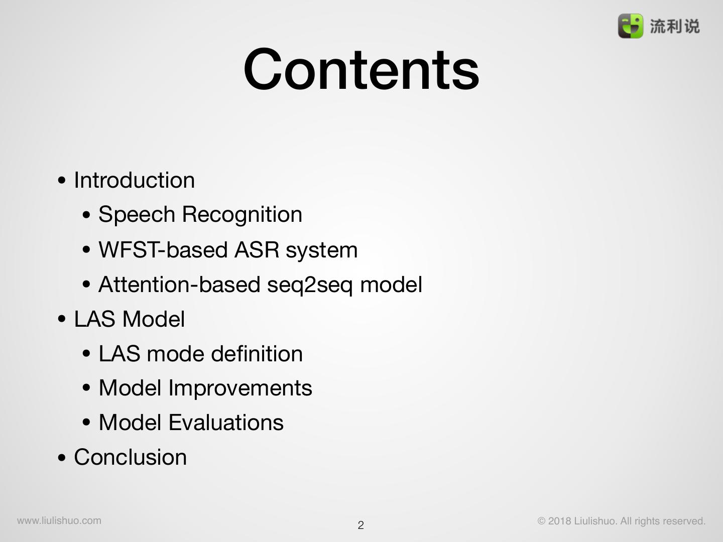
2 . Contents • Introduction • Speech Recognition • WFST-based ASR system • Attention-based seq2seq model • LAS Model • LAS mode definition • Model Improvements • Model Evaluations • Conclusion www.liulishuo.com !2 © 2018 Liulishuo. All rights reserved.

3 . Contents • Introduction • Speech Recognition • WFST-based ASR system • Attention-based seq2seq model • LAS Model • LAS mode definition • Model Improvements • Model Evaluations • Conclusion www.liulishuo.com !3 © 2018 Liulishuo. All rights reserved.

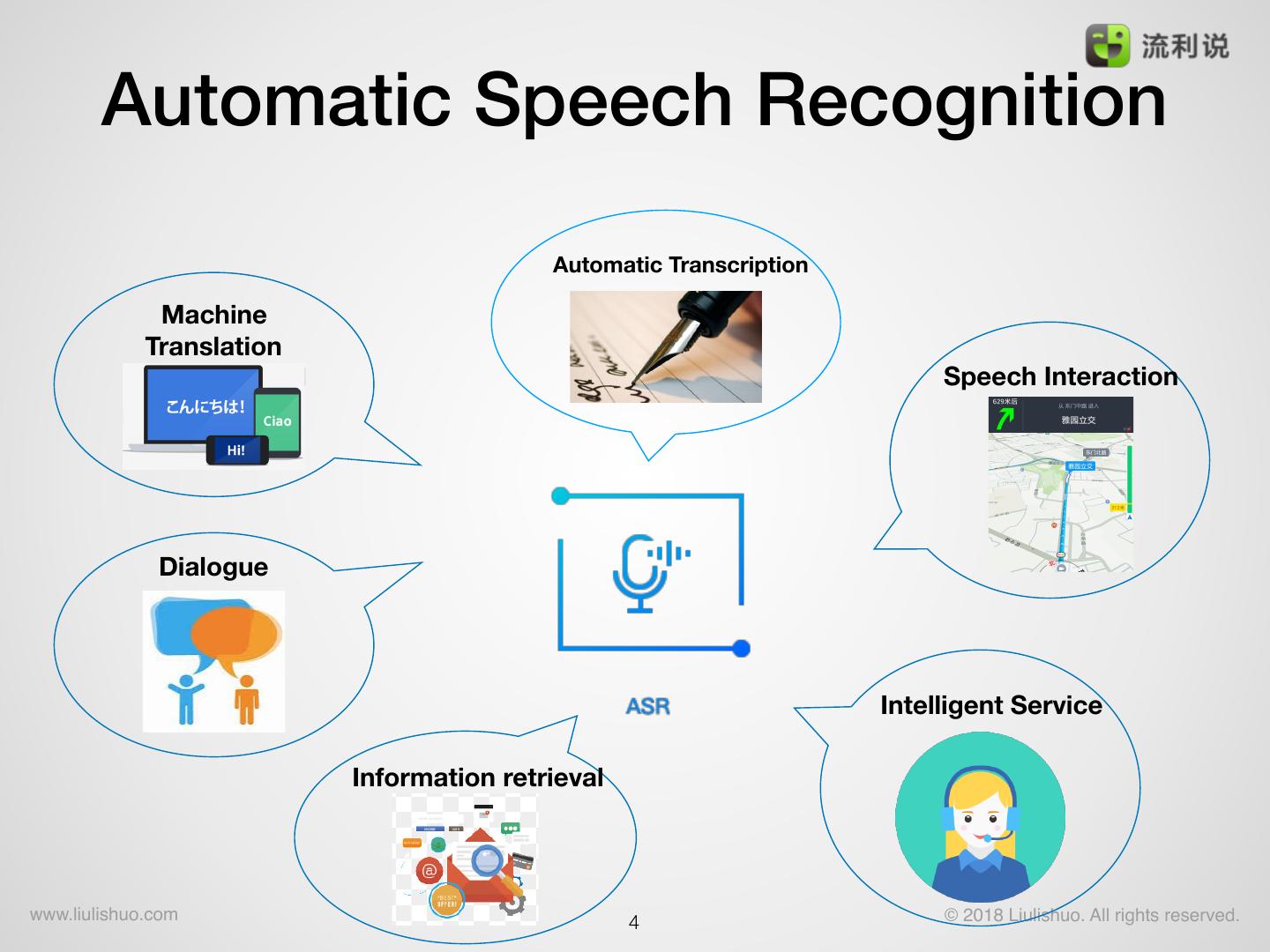
4 . Automatic Speech Recognition Automatic Transcription Machine Translation Speech Interaction Dialogue Intelligent Service Information retrieval www.liulishuo.com !4 © 2018 Liulishuo. All rights reserved.

5 . WFST-based ASR System • Given the speech audio (features), find the optimal word sequence. Decoder O W 明天有空吗？ Formulation: acoustic model language model p(O | W ) ⋅ p(W ) arg max p(W | O) = arg max p(O) www.liulishuo.com !5 © 2018 Liulishuo. All rights reserved.

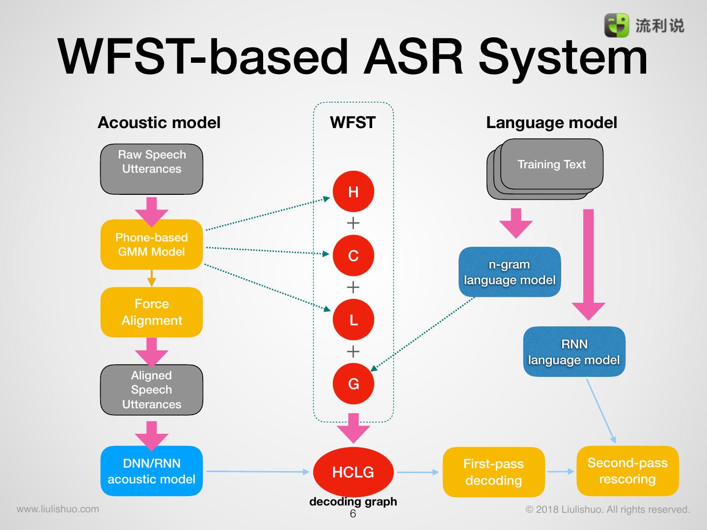
6 . WFST-based ASR System Acoustic model WFST Language model Raw Speech Utterances Training Text H + Phone-based GMM Model C n-gram + language model Force Alignment L + RNN language model Aligned Speech G Utterances DNN/RNN First-pass Second-pass acoustic model HCLG rescoring decoding decoding graph www.liulishuo.com !6 © 2018 Liulishuo. All rights reserved.

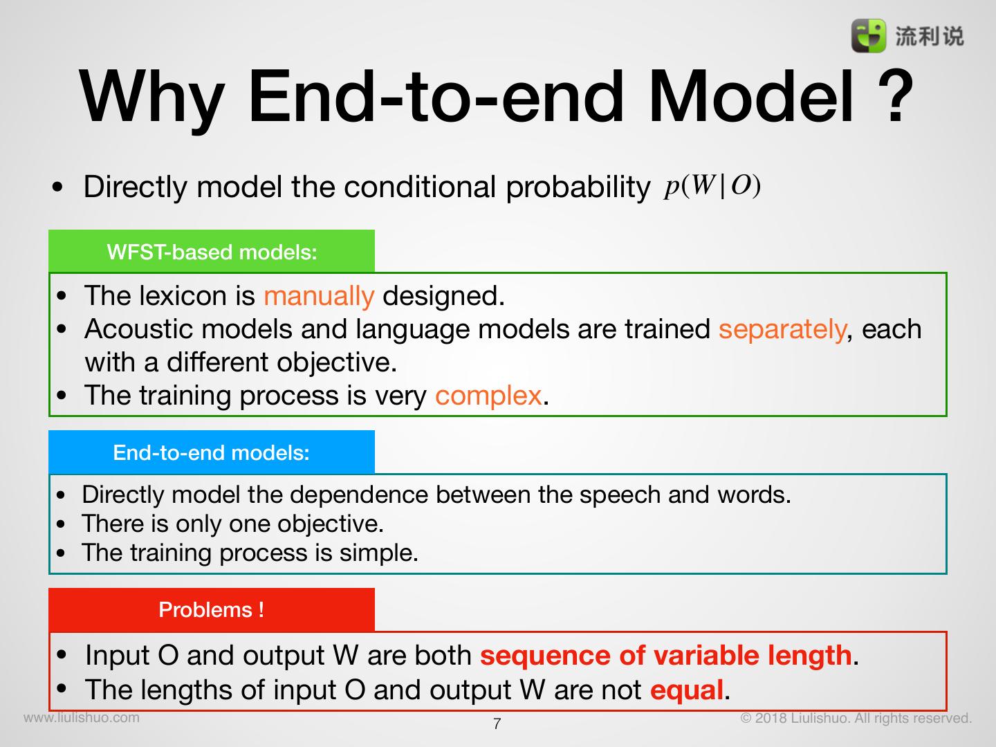
7 . Why End-to-end Model ? • Directly model the conditional probability p(W | O) WFST-based models: • The lexicon is manually designed. • Acoustic models and language models are trained separately, each with a diﬀerent objective. • The training process is very complex. End-to-end models: • Directly model the dependence between the speech and words. • There is only one objective. • The training process is simple. Problems ! • Input O and output W are both sequence of variable length. • The lengths of input O and output W are not equal. www.liulishuo.com © 2018 Liulishuo. All rights reserved. !7

8 . Sequence-to-sequence models • Sequence-to-sequence (Seq2seq) models are based on the encoder-decoder mechanism. • Encoder: encode the input sequence into a fix-length vector • Decoder: decode the fix-length vector to a new sequence • The lengths of the input and output sequences are commonly not equal, and there is no alignment. Output sequence Decoder Vector Encoder Input sequence www.liulishuo.com !8 © 2018 Liulishuo. All rights reserved.

9 . A simple seq2seq model • An encoder RNN to map the sequential variable-length input into a fixed-length vector • A decoder RNN then uses this vector to produce the variable-length output sequence, one token at a time. It’s hard to simply use a hidden vector of RNN to encode the whole sentence. the decoder RNN tends to forget the encoded vector with the output length increasing. Cannot model the alignments ! The encoded vector serves as the initial hidden vector of the decoder RNN Decode until meeting the <eos> end-of-sentence symbol. www.liulishuo.com !9 © 2018 Liulishuo. All rights reserved.

10 . Attention mechanism • Attention in machine translation: 桌上有⼀一只猫 s1 s2 s3 s4 桌上有⼀一只猫 There is a caton the table h1 h2 h3 h4 h5 h6 h7 There is a cat on the table www.liulishuo.com !10 © 2018 Liulishuo. All rights reserved.

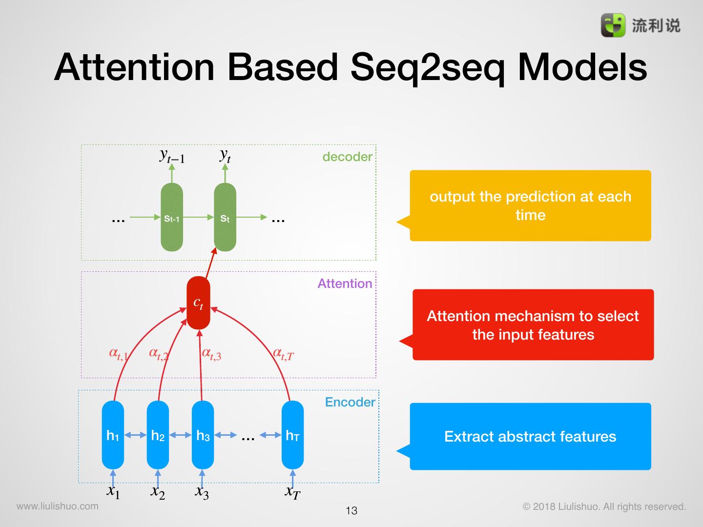
12 . Attention mechanism yt−1 yt Context vector : weighted summary all the encoder hidden vector. … st-1 st … T ∑ ct = αt,ihi i=1 Attention ct Weighted factor : αt,1 αt,2 αt,3 αt,T et,i = NN(st−1, hi) exp(et,i) αt,i = T h1 h2 h3 … hT ∑k=1 exp(et,k) ① Bahdanau, Dzmitry, Kyunghyun Cho, and Yoshua Bengio. "Neural x1 x2 x3 xT machine translation by jointly learning to align and translate." arXiv preprint arXiv:1409.0473, 2014. www.liulishuo.com !12 © 2018 Liulishuo. All rights reserved.

13 . Attention Based Seq2seq Models yt−1 yt decoder output the prediction at each … st-1 st … time Attention ct Attention mechanism to select the input features αt,1 αt,2 αt,3 αt,T Encoder h1 h2 h3 … hT Extract abstract features x1 x2 x3 xT www.liulishuo.com !13 © 2018 Liulishuo. All rights reserved.

14 . Contents • Introduction • Speech Recognition • WFST-based ASR system • Attention-based seq2seq model • LAS Model • LAS mode definition • Model Improvements • Model Evaluations • Conclusion www.liulishuo.com !14 © 2018 Liulishuo. All rights reserved.

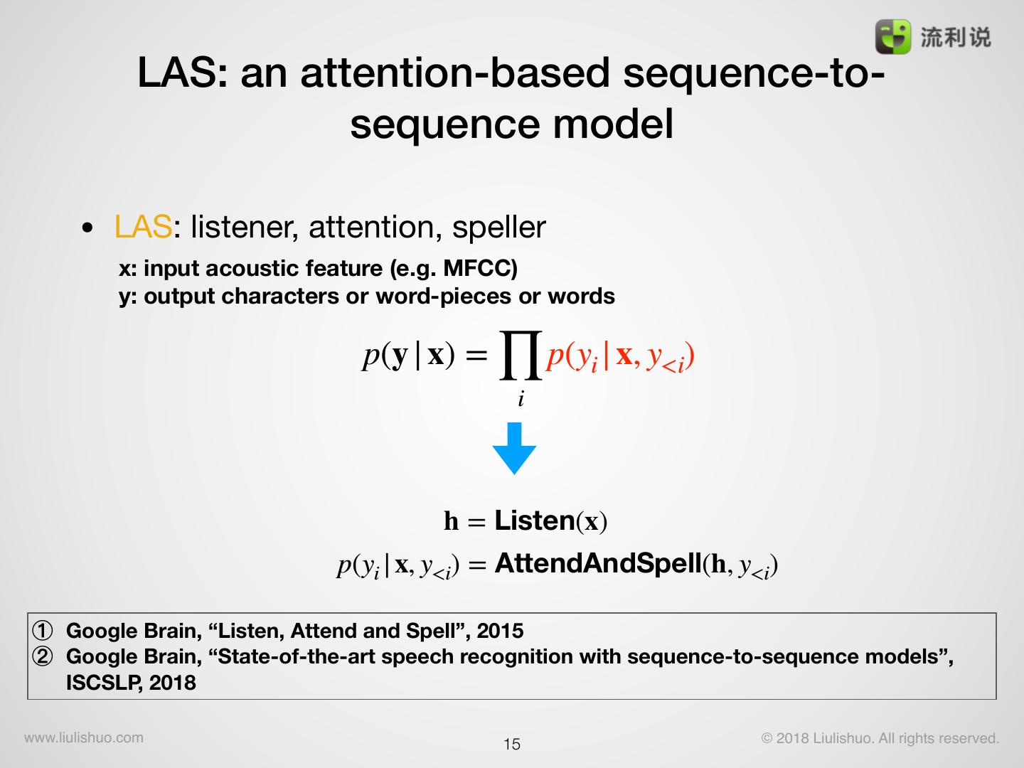
15 . LAS: an attention-based sequence-to- sequence model • LAS: listener, attention, speller x: input acoustic feature (e.g. MFCC) y: output characters or word-pieces or words ∏ p(y | x) = p(yi | x, y<i) i h = Listen(x) p(yi | x, y<i) = AttendAndSpell(h, y<i) ① Google Brain, “Listen, Attend and Spell”, 2015 ② Google Brain, “State-of-the-art speech recognition with sequence-to-sequence models”, ISCSLP, 2018 www.liulishuo.com !15 © 2018 Liulishuo. All rights reserved.

16 . Overview of LAS Model LAS : listener, attention, speller Attention + Decoder: Encoder: Pyramidal BLSTM • Reduce the time resolution • Bidirectional dependence ① Google Brain, “Listen, Attend and Spell”, 2015 www.liulishuo.com !16 © 2018 Liulishuo. All rights reserved.

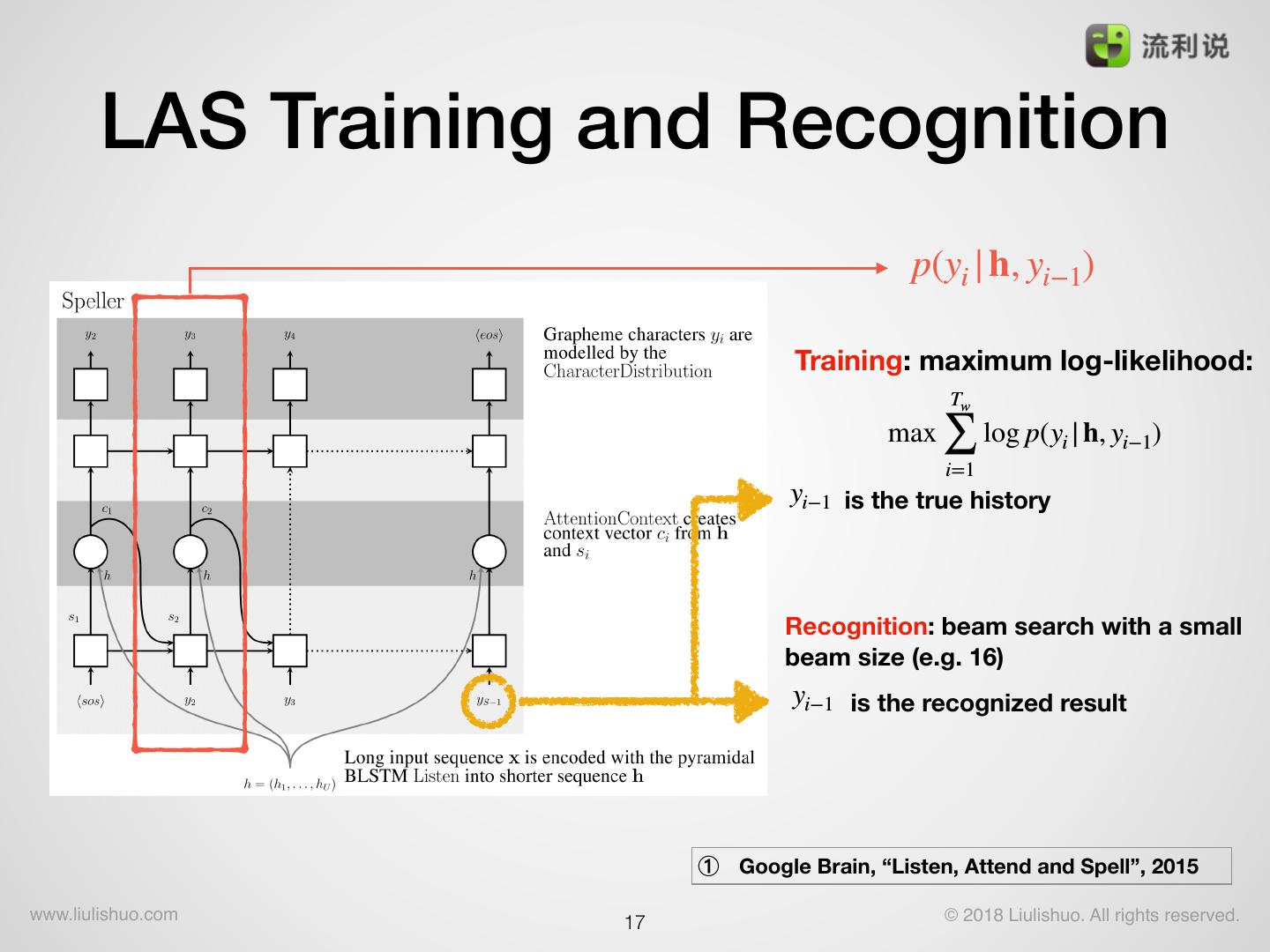
17 . LAS Training and Recognition p(yi | h, yi−1) Training: maximum log-likelihood: Tw ∑ max log p(yi | h, yi−1) i=1 yi−1 is the true history Recognition: beam search with a small beam size (e.g. 16) yi−1 is the recognized result ① Google Brain, “Listen, Attend and Spell”, 2015 www.liulishuo.com !17 © 2018 Liulishuo. All rights reserved.

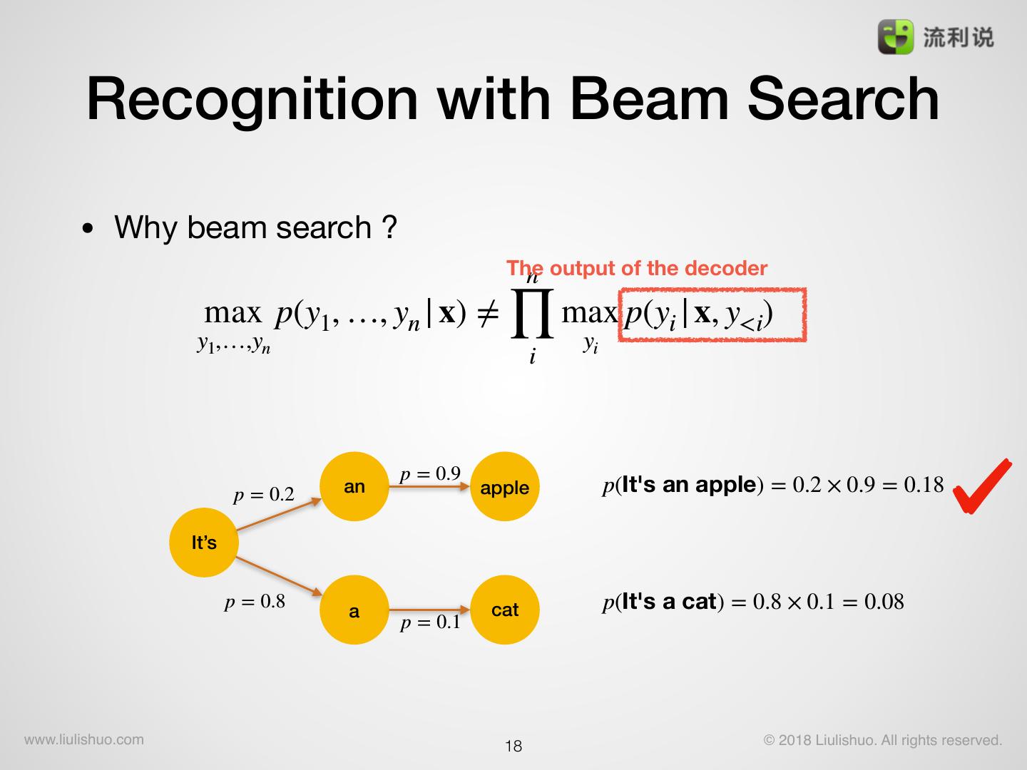
18 . Recognition with Beam Search • Why beam search ? The n output of the decoder ∏ max p(y1, …, yn | x) ≠ max p(yi | x, y<i) y1,…,yn yi i p = 0.9 p = 0.2 an apple p(It's an apple) = 0.2 × 0.9 = 0.18 It’s p = 0.8 a cat p(It's a cat) = 0.8 × 0.1 = 0.08 p = 0.1 www.liulishuo.com !18 © 2018 Liulishuo. All rights reserved.

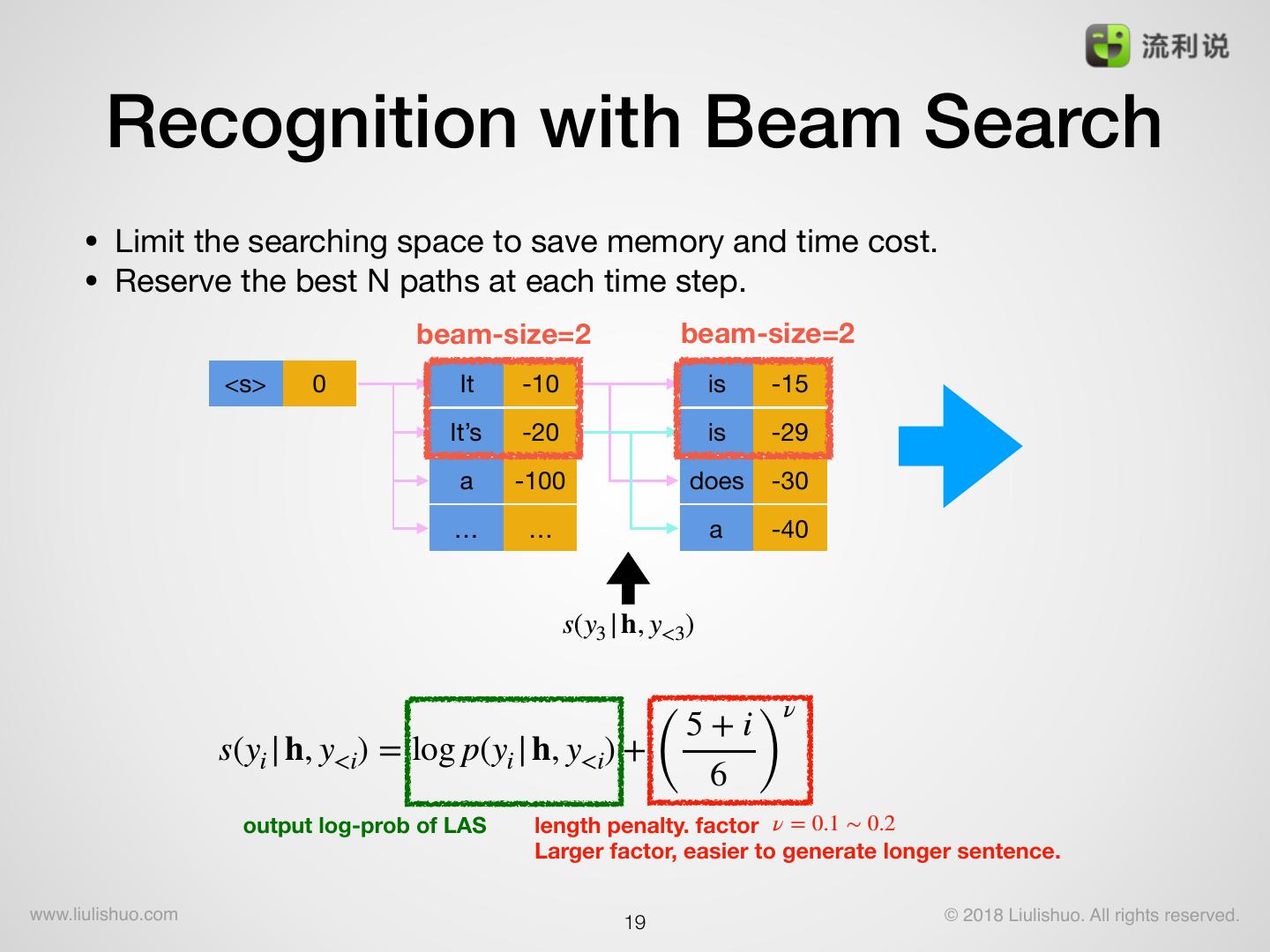
19 . Recognition with Beam Search • Limit the searching space to save memory and time cost. • Reserve the best N paths at each time step. beam-size=2 beam-size=2 <s> 0 It -10 is -15 It’s -20 is -29 a -100 does -30 … … a -40 s(y3 | h, y<3) ( 6 ) ν 5+i s(yi | h, y<i) = log p(yi | h, y<i) + output log-prob of LAS length penalty. factor ν = 0.1 ∼ 0.2 Larger factor, easier to generate longer sentence. www.liulishuo.com !19 © 2018 Liulishuo. All rights reserved.

20 . Improvements: word piece • Character/Word output -> word-piece (subword) output The automatic algorithm based on a simple data compression technique - Byte Pair Encoding (BPE), that iteratively replaces the most frequent pair of bytes in a sequence with a single, unused byte. • over character: reduce the output length and improve the performance • over word: reduce the output dimension and avoid the OOV problems. merge new wp count e+r er 5 new. 1 er + . er. 5 [new] [.] newer. 3 n+e ne 4 [newer.] wider. 2 ne + w new 4 [w] [i] [d] [er.] new + er. newer. 3 … … … [1] Sennrich, Rico, Barry Haddow, and Alexandra Birch. "Neural machine translation of rare words with subword units." arXiv preprint arXiv:1508.07909, 2015. www.liulishuo.com !20 © 2018 Liulishuo. All rights reserved.

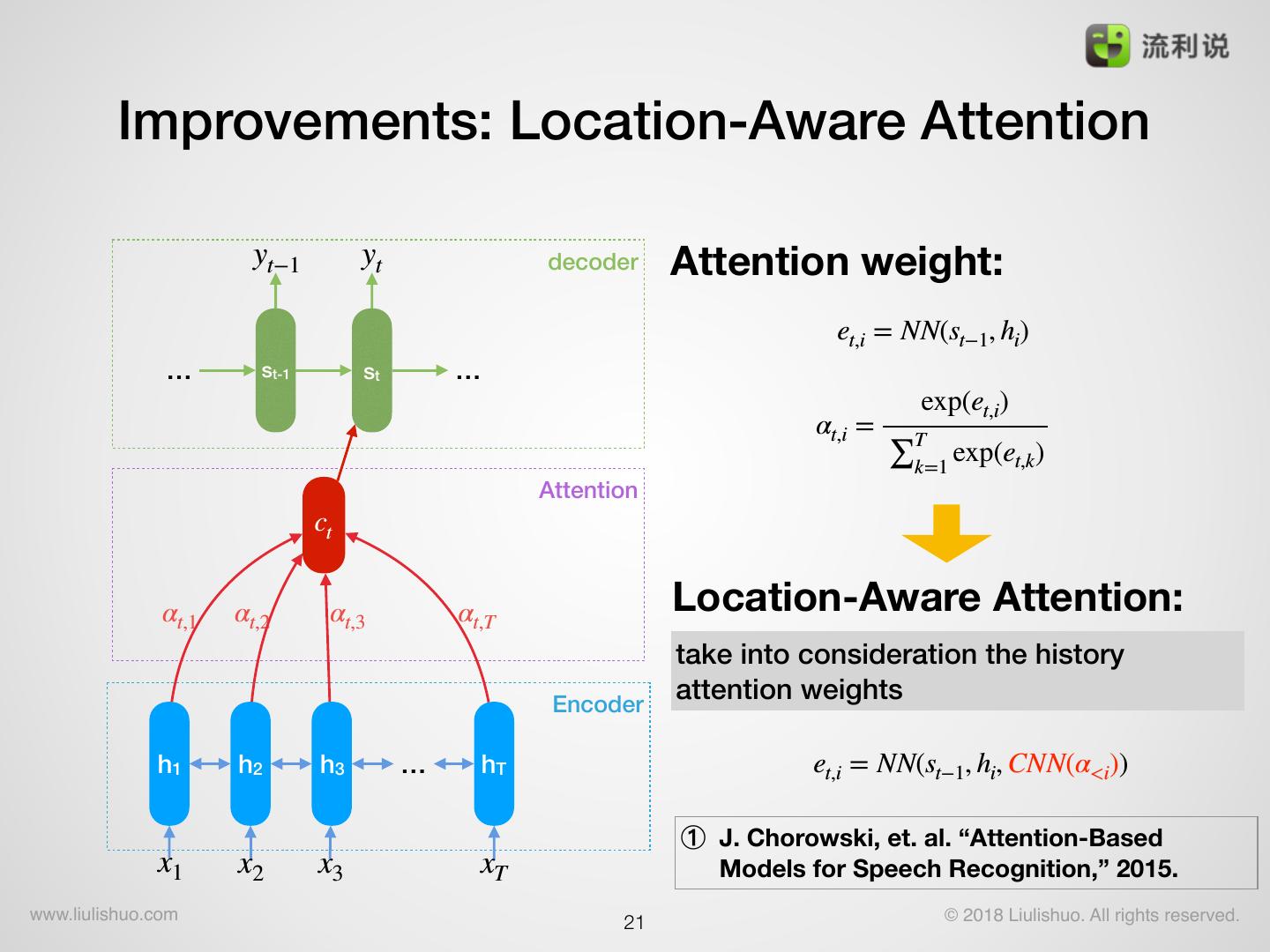
21 . Improvements: Location-Aware Attention yt−1 yt decoder Attention weight: et,i = NN(st−1, hi) … st-1 st … exp(et,i) αt,i = T ∑k=1 exp(et,k) Attention ct αt,1 αt,2 αt,3 αt,T Location-Aware Attention: take into consideration the history Encoder attention weights h1 h2 h3 … hT et,i = NN(st−1, hi, CNN(α<i)) ① J. Chorowski, et. al. “Attention-Based x1 x2 x3 xT Models for Speech Recognition,” 2015. www.liulishuo.com !21 © 2018 Liulishuo. All rights reserved.

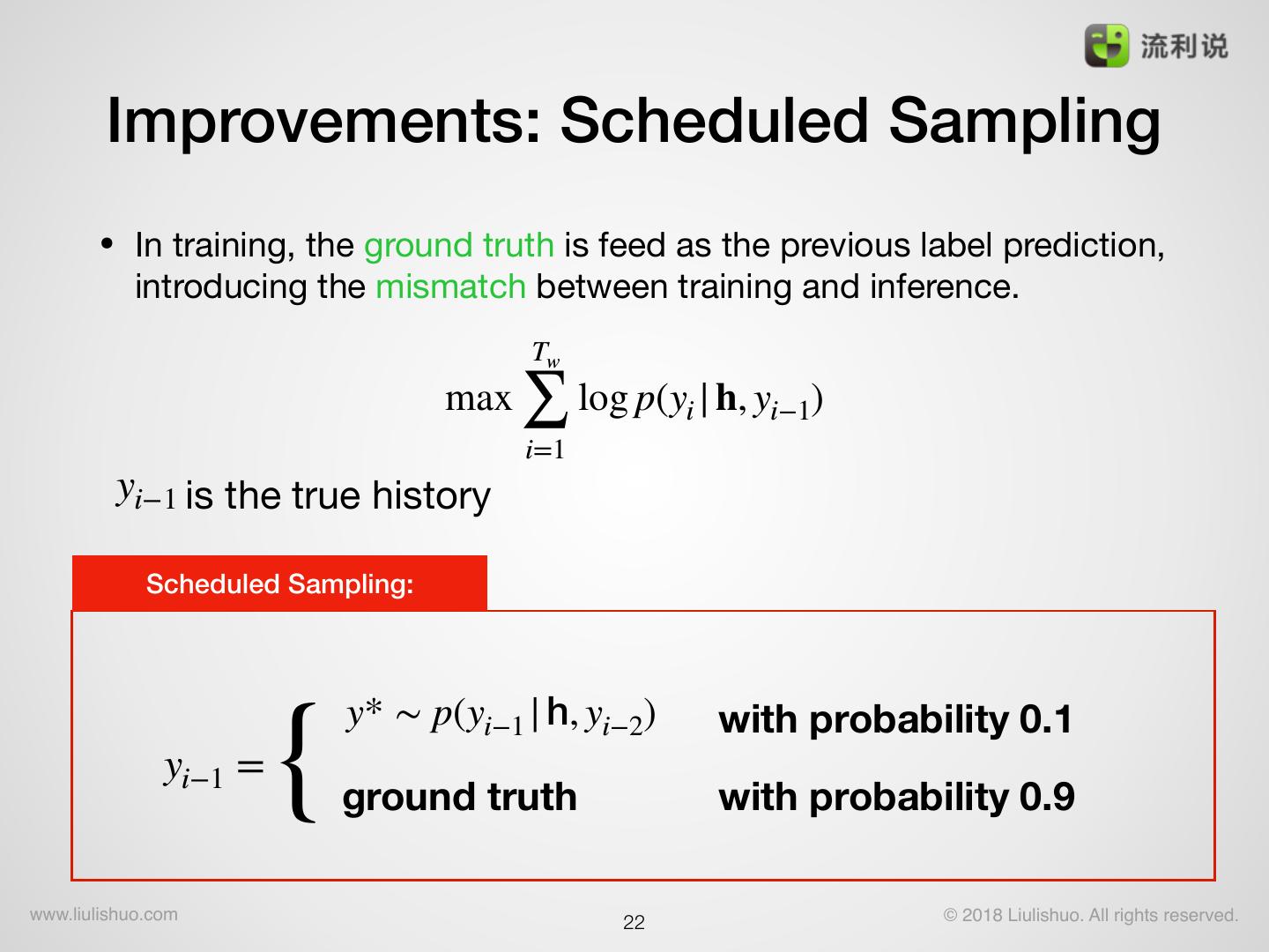
22 . Improvements: Scheduled Sampling • In training, the ground truth is feed as the previous label prediction, introducing the mismatch between training and inference. Tw ∑ max log p(yi | h, yi−1) i=1 yi−1 is the true history Scheduled Sampling: { y* ∼ p(yi−1 | h, yi−2) with probability 0.1 yi−1 = ground truth with probability 0.9 www.liulishuo.com !22 © 2018 Liulishuo. All rights reserved.

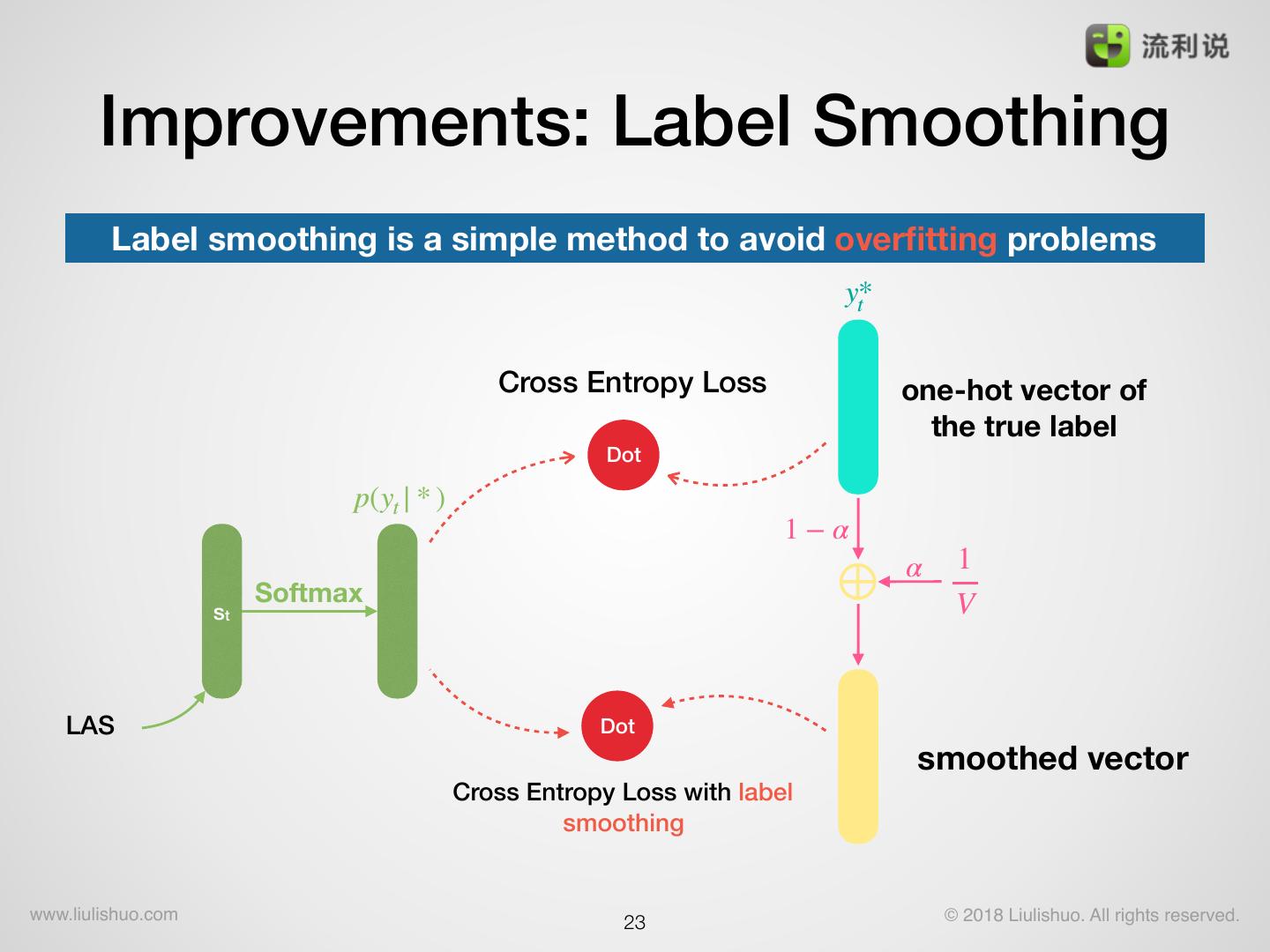
23 . Improvements: Label Smoothing Label smoothing is a simple method to avoid overfitting problems y* t Cross Entropy Loss one-hot vector of the true label Dot p(yt | * ) 1−α 1 Softmax ⊕ α V st LAS Dot smoothed vector Cross Entropy Loss with label smoothing www.liulishuo.com !23 © 2018 Liulishuo. All rights reserved.

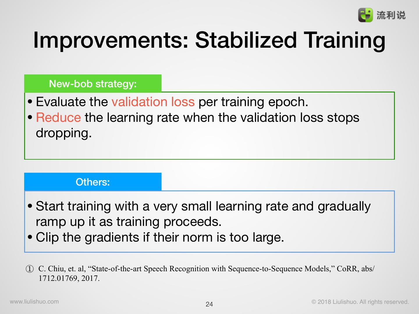
24 . Improvements: Stabilized Training New-bob strategy: • Evaluate the validation loss per training epoch. • Reduce the learning rate when the validation loss stops dropping. Others: • Start training with a very small learning rate and gradually ramp up it as training proceeds. • Clip the gradients if their norm is too large. ① C. Chiu, et. al, “State-of-the-art Speech Recognition with Sequence-to-Sequence Models,” CoRR, abs/ 1712.01769, 2017. www.liulishuo.com !24 © 2018 Liulishuo. All rights reserved.

25 . Improvements: Data Augmentation To balance the datas coming from different domains. duration of ASR training datas（hours） } native-readaloud nonnative-readaloud-v1 randomly select the audio nonnative-readaloud-v2 nonnative-readaloud-v3 } TEDLIUM_release1 telis-asr-v3 change the speed based telis-asr-v4 ratio=0.9, 0.95, 1.0, 1.05, 1.1 chatbot-02 0 500 1,000 1,500 2,000 2,500 3,000 3,500 4,000 4,500 5,000 total duration selected duration www.liulishuo.com !25 © 2018 Liulishuo. All rights reserved.

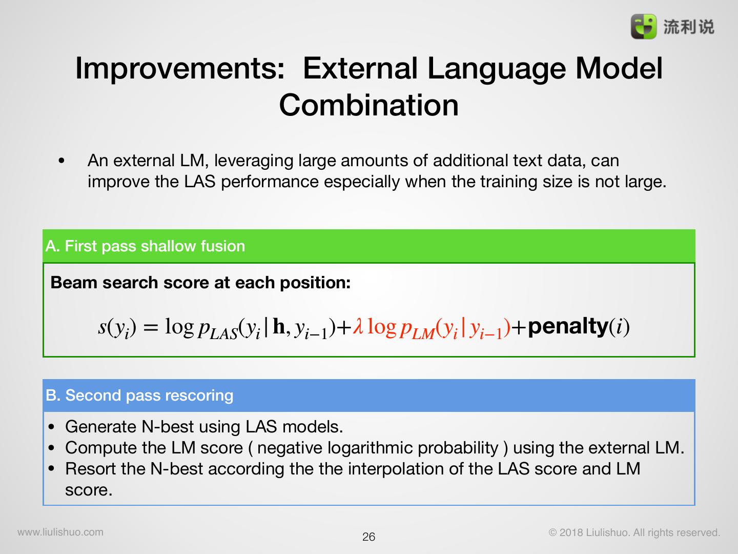
26 . Improvements: External Language Model Combination • An external LM, leveraging large amounts of additional text data, can improve the LAS performance especially when the training size is not large. A. First pass shallow fusion Beam search score at each position: s(yi) = log pLAS(yi | h, yi−1)+λ log pLM(yi | yi−1)+penalty(i) B. Second pass rescoring • Generate N-best using LAS models. • Compute the LM score ( negative logarithmic probability ) using the external LM. • Resort the N-best according the the interpolation of the LAS score and LM score. www.liulishuo.com !26 © 2018 Liulishuo. All rights reserved.

27 . WER results on LibriSpeech • 1000 hours training speech. • 40-dim static filter-bank features. • encoder: 3 pyramid BLSTM with 1024 hidden units. • decoder: 2 LSTM with 512 hidden units. • word-piece size is 500. • All the improvements are used. DEV-clean Test-clean WERR LAS no external LM 4.21 4.34 + 4gram LM rescore 3.52 3.76 13.4% + LSTM LM rescore 3.33 3.57 17.7% + LSTM LM shallow fusion 3.17 3.43 21.0% www.liulishuo.com !27 © 2018 Liulishuo. All rights reserved.

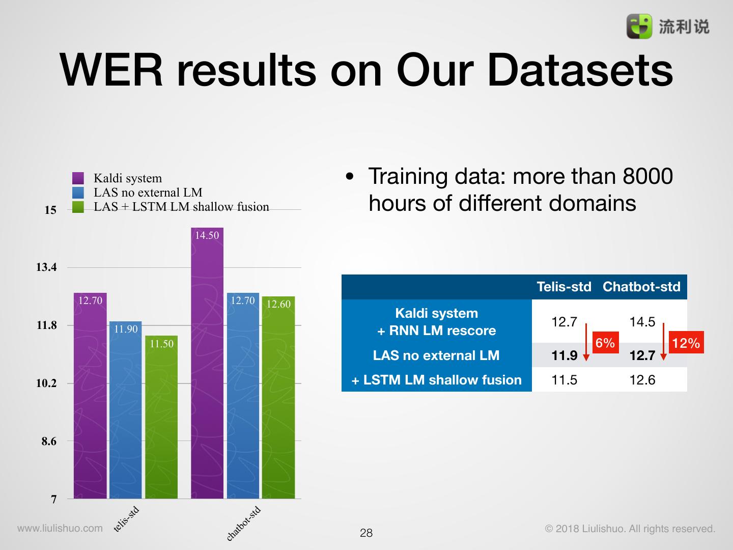
28 . WER results on Our Datasets Kaldi system LAS no external LM • Training data: more than 8000 15 LAS + LSTM LM shallow fusion hours of diﬀerent domains 14.50 13.4 Telis-std Chatbot-std 12.70 12.70 12.60 Kaldi system 11.8 12.7 14.5 11.90 + RNN LM rescore 11.50 6% 12% LAS no external LM 11.9 12.7 10.2 + LSTM LM shallow fusion 11.5 12.6 8.6 7 std td t-s - lis bo www.liulishuo.com !28 © 2018 Liulishuo. All rights reserved. te at ch

29 . Contents • Introduction • Speech Recognition • WFST-based ASR system • Attention-based seq2seq model • LAS Model • LAS mode definition • Model Improvements • Model Evaluations • Conclusion www.liulishuo.com !29 © 2018 Liulishuo. All rights reserved.

0点赞

0收藏

7下载