Classification and Regression Trees

1 . Classification and Regression Trees 36-350, Data Mining 6 November 2009 Contents 1 Prediction Trees 1 2 Regression Trees 4 2.1 Example: California Real Estate Again . . . . . . . . . . . . . . . 4 2.2 Regression Tree Fitting . . . . . . . . . . . . . . . . . . . . . . . 7 2.2.1 Cross-Validation and Pruning in R . . . . . . . . . . . . . 13 2.3 Uncertainty in Regression Trees . . . . . . . . . . . . . . . . . . . 14 3 Classification Trees 18 3.1 Measuring Information . . . . . . . . . . . . . . . . . . . . . . . . 19 3.2 Making Predictions . . . . . . . . . . . . . . . . . . . . . . . . . . 20 3.3 Measuring Error . . . . . . . . . . . . . . . . . . . . . . . . . . . 20 3.3.1 Misclassification Rate . . . . . . . . . . . . . . . . . . . . 20 3.3.2 Average Loss . . . . . . . . . . . . . . . . . . . . . . . . . 21 3.3.3 Likelihood and Cross-Entropy . . . . . . . . . . . . . . . . 21 3.3.4 Neyman-Pearson Approach . . . . . . . . . . . . . . . . . 23 4 Further Reading 24 5 Exercises 24 Reading: Principles of Data Mining, sections 10.5 and 5.2 (in that order); Berk, chapter 3 Having built up increasingly complicated models for regression, I’ll now switch gears and introduce a class of nonlinear predictive model which at first seems too simple to possible work, namely prediction trees. These have two varieties, regression trees and classification trees. 1 Prediction Trees The basic idea is very simple. We want to predict a response or class Y from inputs X1 , X2 , . . . Xp . We do this by growing a binary tree. At each internal 1 

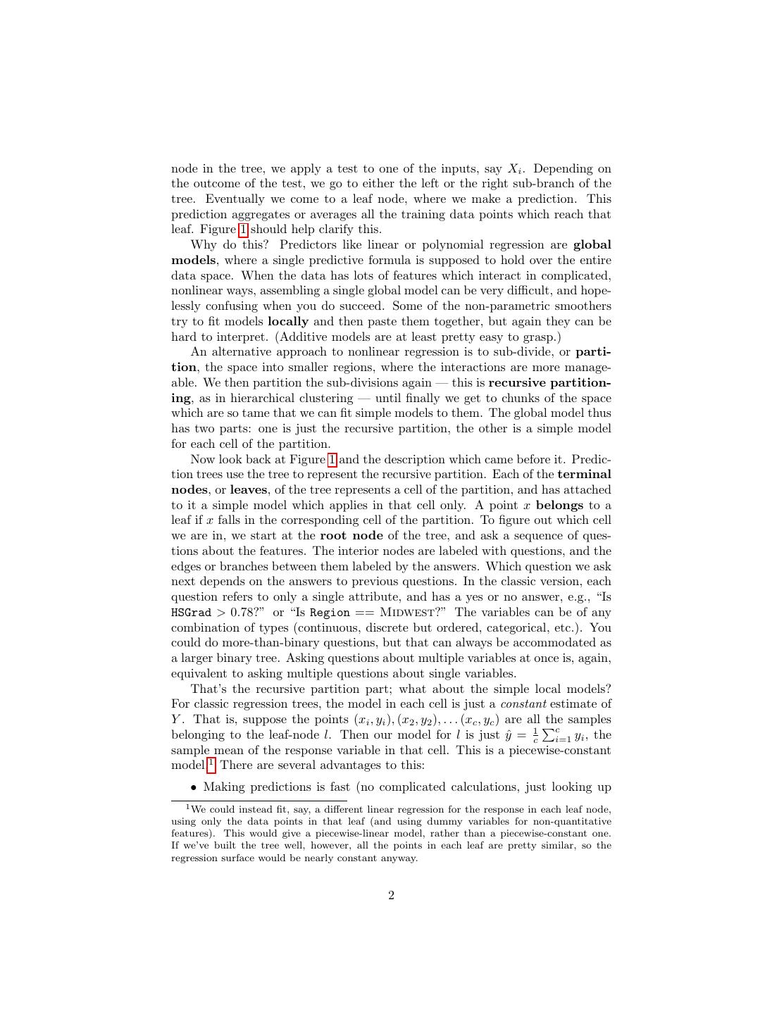
2 .node in the tree, we apply a test to one of the inputs, say Xi . Depending on the outcome of the test, we go to either the left or the right sub-branch of the tree. Eventually we come to a leaf node, where we make a prediction. This prediction aggregates or averages all the training data points which reach that leaf. Figure 1 should help clarify this. Why do this? Predictors like linear or polynomial regression are global models, where a single predictive formula is supposed to hold over the entire data space. When the data has lots of features which interact in complicated, nonlinear ways, assembling a single global model can be very difficult, and hope- lessly confusing when you do succeed. Some of the non-parametric smoothers try to fit models locally and then paste them together, but again they can be hard to interpret. (Additive models are at least pretty easy to grasp.) An alternative approach to nonlinear regression is to sub-divide, or parti- tion, the space into smaller regions, where the interactions are more manage- able. We then partition the sub-divisions again — this is recursive partition- ing, as in hierarchical clustering — until finally we get to chunks of the space which are so tame that we can fit simple models to them. The global model thus has two parts: one is just the recursive partition, the other is a simple model for each cell of the partition. Now look back at Figure 1 and the description which came before it. Predic- tion trees use the tree to represent the recursive partition. Each of the terminal nodes, or leaves, of the tree represents a cell of the partition, and has attached to it a simple model which applies in that cell only. A point x belongs to a leaf if x falls in the corresponding cell of the partition. To figure out which cell we are in, we start at the root node of the tree, and ask a sequence of ques- tions about the features. The interior nodes are labeled with questions, and the edges or branches between them labeled by the answers. Which question we ask next depends on the answers to previous questions. In the classic version, each question refers to only a single attribute, and has a yes or no answer, e.g., “Is HSGrad > 0.78?” or “Is Region == Midwest?” The variables can be of any combination of types (continuous, discrete but ordered, categorical, etc.). You could do more-than-binary questions, but that can always be accommodated as a larger binary tree. Asking questions about multiple variables at once is, again, equivalent to asking multiple questions about single variables. That’s the recursive partition part; what about the simple local models? For classic regression trees, the model in each cell is just a constant estimate of Y . That is, suppose the points (xi , yi ), (x2 , y2 ), . . . (xc , yc ) are all the samples c belonging to the leaf-node l. Then our model for l is just yˆ = 1c i=1 yi , the sample mean of the response variable in that cell. This is a piecewise-constant model.1 There are several advantages to this: • Making predictions is fast (no complicated calculations, just looking up 1 We could instead fit, say, a different linear regression for the response in each leaf node, using only the data points in that leaf (and using dummy variables for non-quantitative features). This would give a piecewise-linear model, rather than a piecewise-constant one. If we’ve built the tree well, however, all the points in each leaf are pretty similar, so the regression surface would be nearly constant anyway. 2 

3 .Figure 1: Classification tree for county-level outcomes in the 2008 Democratic Party primary (as of April 16), by Amanada Cox for the New York Times. 3 

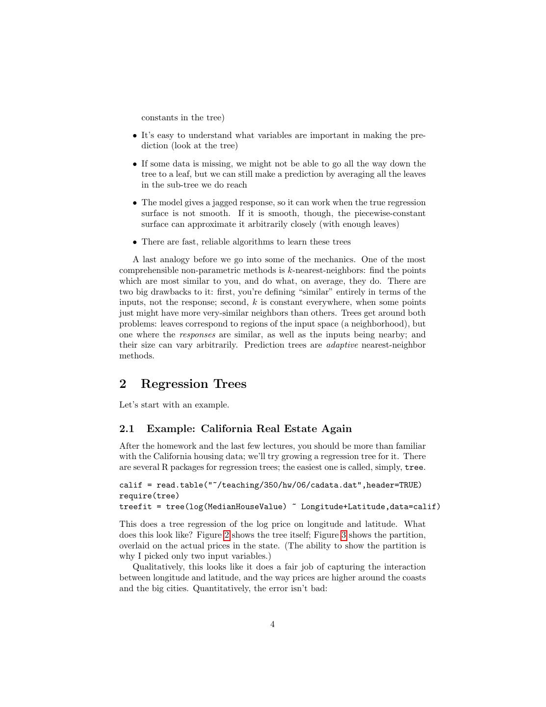
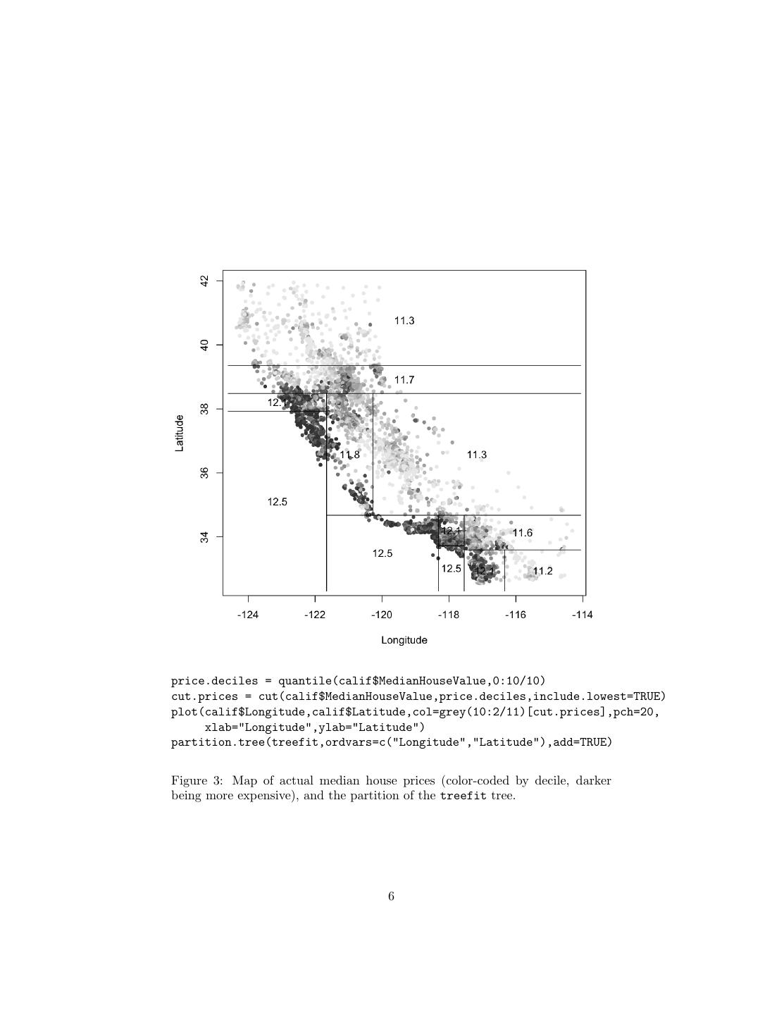
4 . constants in the tree) • It’s easy to understand what variables are important in making the pre- diction (look at the tree) • If some data is missing, we might not be able to go all the way down the tree to a leaf, but we can still make a prediction by averaging all the leaves in the sub-tree we do reach • The model gives a jagged response, so it can work when the true regression surface is not smooth. If it is smooth, though, the piecewise-constant surface can approximate it arbitrarily closely (with enough leaves) • There are fast, reliable algorithms to learn these trees A last analogy before we go into some of the mechanics. One of the most comprehensible non-parametric methods is k-nearest-neighbors: find the points which are most similar to you, and do what, on average, they do. There are two big drawbacks to it: first, you’re defining “similar” entirely in terms of the inputs, not the response; second, k is constant everywhere, when some points just might have more very-similar neighbors than others. Trees get around both problems: leaves correspond to regions of the input space (a neighborhood), but one where the responses are similar, as well as the inputs being nearby; and their size can vary arbitrarily. Prediction trees are adaptive nearest-neighbor methods. 2 Regression Trees Let’s start with an example. 2.1 Example: California Real Estate Again After the homework and the last few lectures, you should be more than familiar with the California housing data; we’ll try growing a regression tree for it. There are several R packages for regression trees; the easiest one is called, simply, tree. calif = read.table("~/teaching/350/hw/06/cadata.dat",header=TRUE) require(tree) treefit = tree(log(MedianHouseValue) ~ Longitude+Latitude,data=calif) This does a tree regression of the log price on longitude and latitude. What does this look like? Figure 2 shows the tree itself; Figure 3 shows the partition, overlaid on the actual prices in the state. (The ability to show the partition is why I picked only two input variables.) Qualitatively, this looks like it does a fair job of capturing the interaction between longitude and latitude, and the way prices are higher around the coasts and the big cities. Quantitatively, the error isn’t bad: 4 

5 . Latitude < 38.485 | Longitude < -121.655 Latitude < 39.355 11.73 11.32 Latitude < 37.925 Latitude < 34.675 12.48 12.10 Longitude < -118.315 Longitude < -120.275 11.75 11.28 Longitude < -117.545 12.53 Latitude < 33.725 Latitude < 33.59 Longitude < -116.33 12.54 12.14 11.63 12.09 11.16 plot(treefit) text(treefit,cex=0.75) Figure 2: Regression tree for predicting California housing prices from geo- graphic coordinates. At each internal node, we ask the associated question, and go to the left child if the answer is “yes”, to the right child if the answer is “no”. Note that leaves are labeled with log prices; the plotting function isn’t flexible enough, unfortunately, to apply transformations to the labels. 5 

6 .price.deciles = quantile(calif$MedianHouseValue,0:10/10) cut.prices = cut(calif$MedianHouseValue,price.deciles,include.lowest=TRUE) plot(calif$Longitude,calif$Latitude,col=grey(10:2/11)[cut.prices],pch=20, xlab="Longitude",ylab="Latitude") partition.tree(treefit,ordvars=c("Longitude","Latitude"),add=TRUE) Figure 3: Map of actual median house prices (color-coded by decile, darker being more expensive), and the partition of the treefit tree. 6 

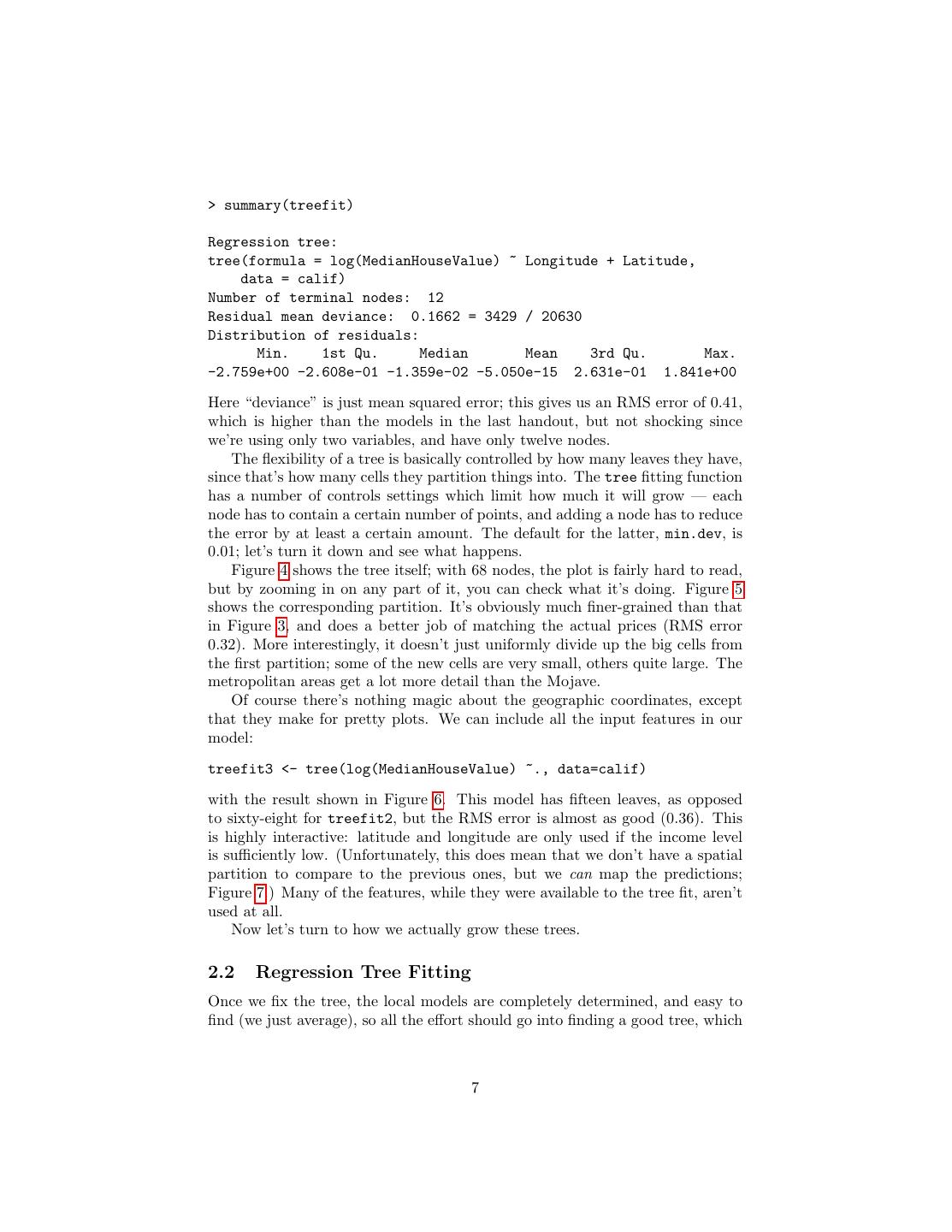
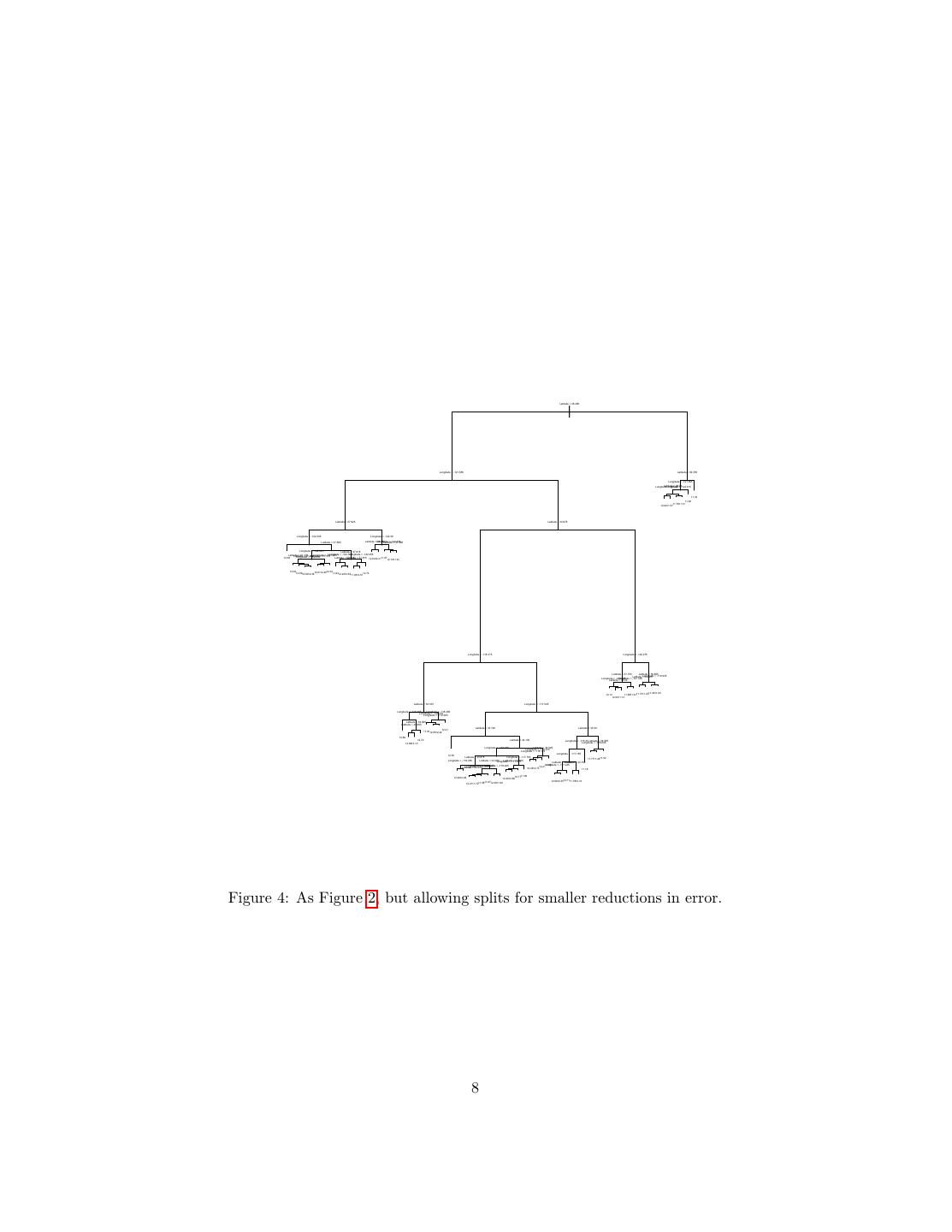
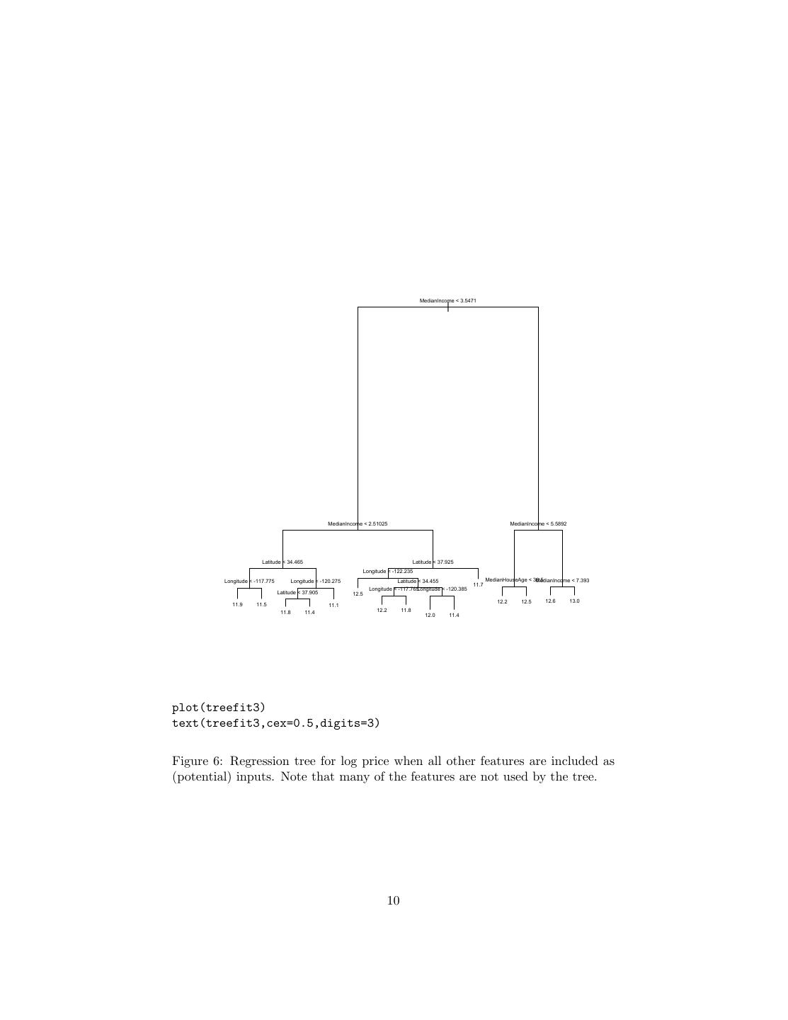
7 .> summary(treefit) Regression tree: tree(formula = log(MedianHouseValue) ~ Longitude + Latitude, data = calif) Number of terminal nodes: 12 Residual mean deviance: 0.1662 = 3429 / 20630 Distribution of residuals: Min. 1st Qu. Median Mean 3rd Qu. Max. -2.759e+00 -2.608e-01 -1.359e-02 -5.050e-15 2.631e-01 1.841e+00 Here “deviance” is just mean squared error; this gives us an RMS error of 0.41, which is higher than the models in the last handout, but not shocking since we’re using only two variables, and have only twelve nodes. The flexibility of a tree is basically controlled by how many leaves they have, since that’s how many cells they partition things into. The tree fitting function has a number of controls settings which limit how much it will grow — each node has to contain a certain number of points, and adding a node has to reduce the error by at least a certain amount. The default for the latter, min.dev, is 0.01; let’s turn it down and see what happens. Figure 4 shows the tree itself; with 68 nodes, the plot is fairly hard to read, but by zooming in on any part of it, you can check what it’s doing. Figure 5 shows the corresponding partition. It’s obviously much finer-grained than that in Figure 3, and does a better job of matching the actual prices (RMS error 0.32). More interestingly, it doesn’t just uniformly divide up the big cells from the first partition; some of the new cells are very small, others quite large. The metropolitan areas get a lot more detail than the Mojave. Of course there’s nothing magic about the geographic coordinates, except that they make for pretty plots. We can include all the input features in our model: treefit3 <- tree(log(MedianHouseValue) ~., data=calif) with the result shown in Figure 6. This model has fifteen leaves, as opposed to sixty-eight for treefit2, but the RMS error is almost as good (0.36). This is highly interactive: latitude and longitude are only used if the income level is sufficiently low. (Unfortunately, this does mean that we don’t have a spatial partition to compare to the previous ones, but we can map the predictions; Figure 7.) Many of the features, while they were available to the tree fit, aren’t used at all. Now let’s turn to how we actually grow these trees. 2.2 Regression Tree Fitting Once we fix the tree, the local models are completely determined, and easy to find (we just average), so all the effort should go into finding a good tree, which 7 

8 . Latitude < 38.485 | Longitude < -121.655 Latitude < 39.355 Longitude < -121.365 Latitude < 38.86 Longitude Longitude < -121.57 < -122.915 11.32 11.90 11.7611.31 12.0211.57 Latitude < 37.925 Latitude < 34.675 Longitude < -122.305 Longitude < -122.38 Latitude < 37.585 Latitude < Longitude 38.225 < -122.335 Latitude < 37.985 Longitude < -122.025 Latitude < 37.815 Latitude < 37.175 Longitude < -122.145 Longitude < -121.865 Longitude < -122.255 Latitude Latitude < 37.315 < 37.465 Longitude < -122.235 12.68 Latitude < 37.715 Latitude < 37.875 12.6412.2111.5712.1911.91 12.3912.89 12.32 12.8012.3612.6112.40 11.9312.2312.63 12.73 11.9312.51 Longitude < -118.315 Longitude < -120.275 Latitude < 37.155 Latitude < 36.805 Latitude <Longitude 34.825 < -119.935 Longitude < -120.645 Longitude < -121.335 Latitude < 36.02 11.2911.64 12.14 11.8811.6111.7311.20 12.0011.13 Latitude < 34.165 Longitude < -117.545 Longitude < -118.365 Longitude < -118.485 Longitude < -120.415 Longitude < -119.365 Latitude < 34.055 Latitude < 33.885 Latitude < 33.725 Latitude < 33.59 12.21 11.8112.6512.42 12.86 12.72 Latitude < 34.105 Longitude < -116.33 Latitude < 34.055 Longitude < -116.245 12.6912.10 Longitude < -118.165 Latitude < 34.525 Longitude < -118.015 Longitude < -118.115 Longitude < -117.165 12.54 Latitude < 33.875 Longitude < -117.755 11.7711.2811.52 Longitude < -118.285 Latitude < 34.045 Latitude Longitude < 33.905 < -117.815 Latitude < 33.125 Latitude < 32.755 Longitude < -118.225 Longitude < -118.245 Longitude < -117.235 11.88 Longitude < -118.285 Latitude < 33.915 12.4512.7312.21 11.16 12.4612.08 12.1711.90 12.2612.68 12.1111.7812.10 11.8712.2911.90 12.6912.35 12.2111.7211.58 Figure 4: As Figure 2, but allowing splits for smaller reductions in error. 8 

9 .plot(calif$Longitude,calif$Latitude,col=grey(10:2/11)[cut.prices],pch=20, xlab="Longitude",ylab="Latitude") partition.tree(treefit2,ordvars=c("Longitude","Latitude"),add=TRUE,cex=0.3) Figure 5: Partition for treefit2. Note the high level of detail around the cities, as compared to the much coarser cells covering rural areas where variations in prices are less extreme. 9 

10 . MedianIncome < 3.5471 | MedianIncome < 2.51025 MedianIncome < 5.5892 Latitude < 34.465 Latitude < 37.925 Longitude < -122.235 Longitude < -117.775 Longitude < -120.275 Latitude < 34.455 MedianHouseAge < 38.5 MedianIncome < 7.393 11.7 Longitude < -117.765Longitude < -120.385 Latitude < 37.905 12.5 12.2 12.5 12.6 13.0 11.9 11.5 11.1 11.8 11.4 12.2 11.8 12.0 11.4 plot(treefit3) text(treefit3,cex=0.5,digits=3) Figure 6: Regression tree for log price when all other features are included as (potential) inputs. Note that many of the features are not used by the tree. 10 

11 .cut.predictions = cut(predict(treefit3),log(price.deciles),include.lowest=TRUE) plot(calif$Longitude,calif$Latitude,col=grey(10:2/11)[cut.predictions],pch=20, xlab="Longitude",ylab="Latitude") Figure 7: Predicted prices for the treefit3 model. Same color scale as in previous plots (where dots indicated actual prices). 11 

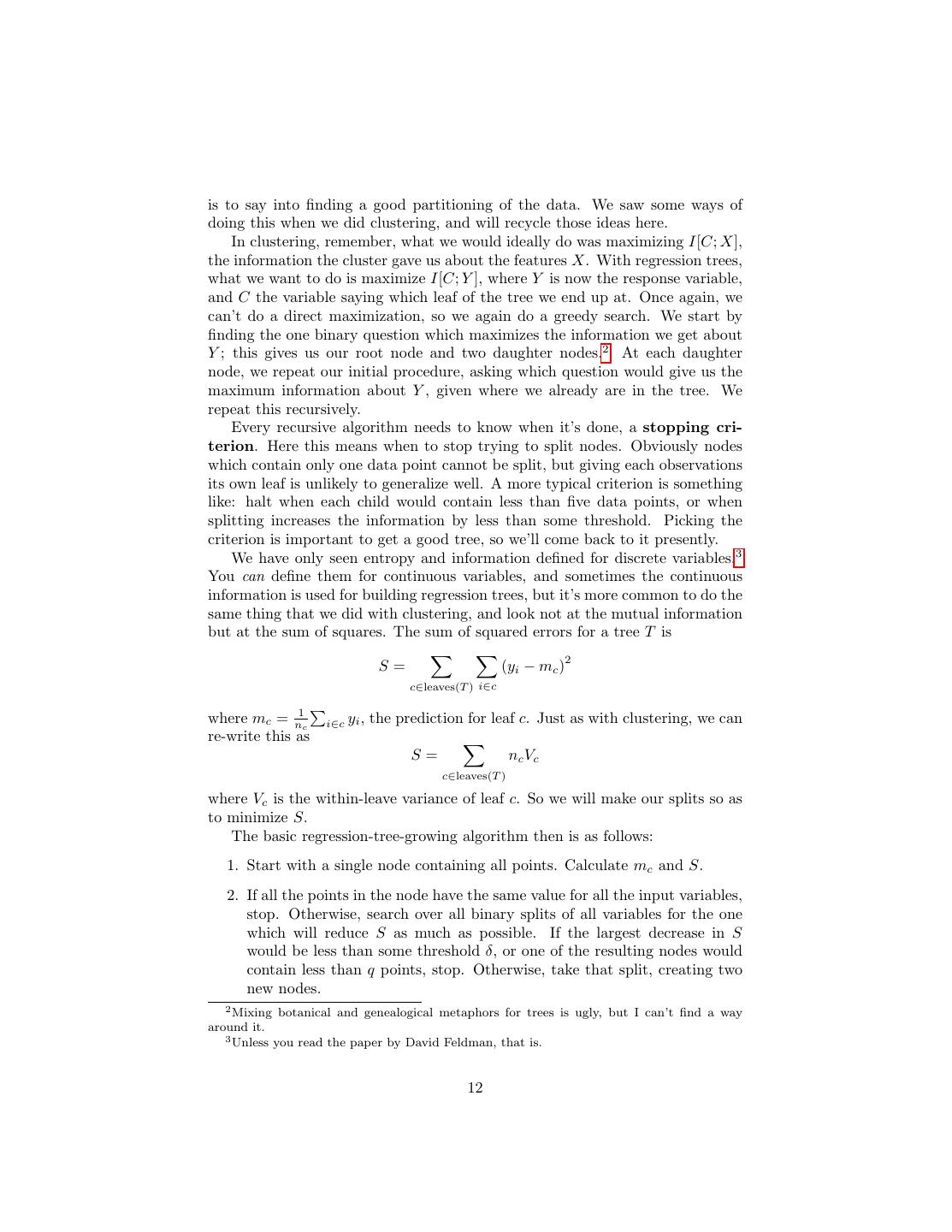
12 .is to say into finding a good partitioning of the data. We saw some ways of doing this when we did clustering, and will recycle those ideas here. In clustering, remember, what we would ideally do was maximizing I[C; X], the information the cluster gave us about the features X. With regression trees, what we want to do is maximize I[C; Y ], where Y is now the response variable, and C the variable saying which leaf of the tree we end up at. Once again, we can’t do a direct maximization, so we again do a greedy search. We start by finding the one binary question which maximizes the information we get about Y ; this gives us our root node and two daughter nodes.2 At each daughter node, we repeat our initial procedure, asking which question would give us the maximum information about Y , given where we already are in the tree. We repeat this recursively. Every recursive algorithm needs to know when it’s done, a stopping cri- terion. Here this means when to stop trying to split nodes. Obviously nodes which contain only one data point cannot be split, but giving each observations its own leaf is unlikely to generalize well. A more typical criterion is something like: halt when each child would contain less than five data points, or when splitting increases the information by less than some threshold. Picking the criterion is important to get a good tree, so we’ll come back to it presently. We have only seen entropy and information defined for discrete variables.3 You can define them for continuous variables, and sometimes the continuous information is used for building regression trees, but it’s more common to do the same thing that we did with clustering, and look not at the mutual information but at the sum of squares. The sum of squared errors for a tree T is 2 S= (yi − mc ) c∈leaves(T ) i∈c where mc = n1c i∈c yi , the prediction for leaf c. Just as with clustering, we can re-write this as S= nc Vc c∈leaves(T ) where Vc is the within-leave variance of leaf c. So we will make our splits so as to minimize S. The basic regression-tree-growing algorithm then is as follows: 1. Start with a single node containing all points. Calculate mc and S. 2. If all the points in the node have the same value for all the input variables, stop. Otherwise, search over all binary splits of all variables for the one which will reduce S as much as possible. If the largest decrease in S would be less than some threshold δ, or one of the resulting nodes would contain less than q points, stop. Otherwise, take that split, creating two new nodes. 2 Mixing botanical and genealogical metaphors for trees is ugly, but I can’t find a way around it. 3 Unless you read the paper by David Feldman, that is. 12 

13 . 3. In each new node, go back to step 1. Trees use only one feature (input variable) at each step. If multiple fea- tures are equally good, which one is chosen is a matter of chance, or arbitrary programming decisions. One problem with the straight-forward algorithm I’ve just given is that it can stop too early, in the following sense. There can be variables which are not very informative themselves, but which lead to very informative subsequent splits. (This was the point of all our talk about interactions when we looked at information theory.) This suggests a problem with stopping when the decrease in S becomes less than some δ. Similar problems can arise from arbitrarily setting a minimum number of points q per node. A more successful approach to finding regression trees uses the idea of cross- validation from last time. We randomly divide our data into a training set and a testing set (say, 50% training and 50% testing). We then apply the basic tree-growing algorithm to the training data only, with q = 1 and δ = 0 — that is, we grow the largest tree we can. This is generally going to be too large and will over-fit the data. We then use cross-validation to prune the tree. At each pair of leaf nodes with a common parent, we evaluate the error on the testing data, and see whether the testing sum of squares would shrink if we removed those two nodes and made their parent a leaf. If so, we prune; if not, not. This is repeated until pruning no longer improves the error on the testing data. The reason this is superior to arbitrary stopping criteria, or to rewarding parsimony as such, is that it directly checks whether the extra capacity (nodes in the tree) pays for itself by improving generalization error. If it does, great; if not, get rid of it. This is something we can do with regression trees that we couldn’t really do with (say) hierarchical clustering, because trees make predictions we can test on new data, and the clustering techniques we looked at before do not. There are lots of other cross-validation tricks for trees. One cute one is to alternate growing and pruning. We divide the data into two parts, as before, and first grow and then prune the tree. We then exchange the role of the training and testing sets, and try to grow our pruned tree to fit the second half. We then prune again, on the first half. We keep alternating in this manner until the size of the tree doesn’t change. 2.2.1 Cross-Validation and Pruning in R The tree package contains functions prune.tree and cv.tree for pruning trees by cross-validation. The function prune.tree takes a tree you fit by tree (see R advice for last homework), and evaluates the error of the tree and various prunings of the tree, all the way down to the stump. The evaluation can be done either on new data, if supplied, or on the training data (the default). If you ask it for a particular size of tree, it gives you the best pruning of that size4 . If you don’t ask it for 4 Or, if there is no tree with that many leaves, the smallest number of leaves ≥ the requested size. 13 

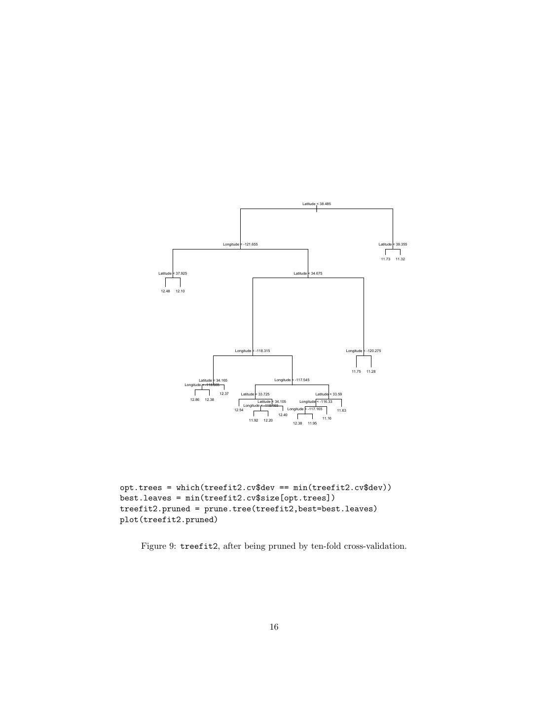
14 .the best tree, it gives an object which shows the number of leaves in the pruned trees, and the error of each one. This object can be plotted. my.tree = tree(y ~ x1 + x2, data=my.data) # Fits tree prune.tree(my.tree,best=5) # Returns best pruned tree with 5 leaves, evaluating # error on training data prune.tree(my.tree,best=5,newdata=test.set) # Ditto, but evaluates on test.set my.tree.seq = prune.tree(my.tree) # Sequence of pruned tree sizes/errors plot(my.tree.seq) # Plots size vs. error my.tree.seq$dev # Vector of error rates for prunings, in order opt.trees = which(my.tree.seq$dev == min(my.tree.seq$dev)) # Positions of # optimal (with respect to error) trees min(my.tree.seq$size[opt.trees]) # Size of smallest optimal tree Finally, prune.tree has an optional method argument. The default is method="deviance", which fits by minimizing the mean squared error (for continuous responses) or the negative log likelihood (for discrete responses; see below).5 The function cv.tree does k-fold cross-validation (default is 10). It requires as an argument a fitted tree, and a function which will take that tree and new data. By default, this function is prune.tree. my.tree.cv = cv.tree(my.tree) The type of output of cv.tree is the same as the function it’s called on. If I do cv.tree(my.tree,best=19) I get the best tree (per cross-validation) of no more than 19 leaves. If I do cv.tree(my.tree) I get information about the cross-validated performance of the whole sequence of pruned trees, e.g., plot(cv.tree(my.tree)). Optional arguments to cv.tree can include K, and any additional arguments for the function it applies. To illustrate, think back to treefit2, which predicted predicted California house prices based on geographic coordinates, but had a very large number of nodes because the tree-growing algorithm was told to split on almost any provocation. Figure 8 shows the size/performance trade-off. Figures 9 and 10 show the result of pruning to the smallest size compatible with minimum cross-validated error. 2.3 Uncertainty in Regression Trees Even when we are making point predictions, we have some uncertainty, because we’ve only seen a finite amount of data, and this is not an entirely representative sample of the underlying probability distribution. With a regression tree, we 5 With discrete responses, you may get better results by saying method="misclass", which looks at the misclassification rate. 14 

15 . 670.0 100.0 66.0 32.0 26.0 16.0 14.0 9.6 8.4 7.7 6500 6000 5500 deviance 5000 4500 4000 3500 1 10 20 30 40 50 60 68 size treefit2.cv <- cv.tree(treefit2) plot(treefit2.cv) Figure 8: Size (horizontal axis) versus cross-validated sum of squared errors (vertical axis) for successive prunings of the treefit2 model. (The upper scale on the horizontal axis refers to the “cost/complexity” penalty. The idea is that the pruning minimizes (total error) + λ(complexity) for a certain value of λ, which is what’s shown on that scale. Here complexity is a function of the number of leaves; see Ripley (1996) for details. Or, just ignore the upper scale!) 15 

16 . Latitude < 38.485 | Longitude < -121.655 Latitude < 39.355 11.73 11.32 Latitude < 37.925 Latitude < 34.675 12.48 12.10 Longitude < -118.315 Longitude < -120.275 11.75 11.28 Latitude < 34.165 Longitude < -117.545 Longitude < -118.365 12.37 Latitude < 33.725 Latitude < 33.59 12.86 12.38 Latitude < 34.105 Longitude < -116.33 Longitude < -118.165 12.54 Longitude < -117.165 11.63 12.40 11.16 11.92 12.20 12.38 11.95 opt.trees = which(treefit2.cv$dev == min(treefit2.cv$dev)) best.leaves = min(treefit2.cv$size[opt.trees]) treefit2.pruned = prune.tree(treefit2,best=best.leaves) plot(treefit2.pruned) Figure 9: treefit2, after being pruned by ten-fold cross-validation. 16 

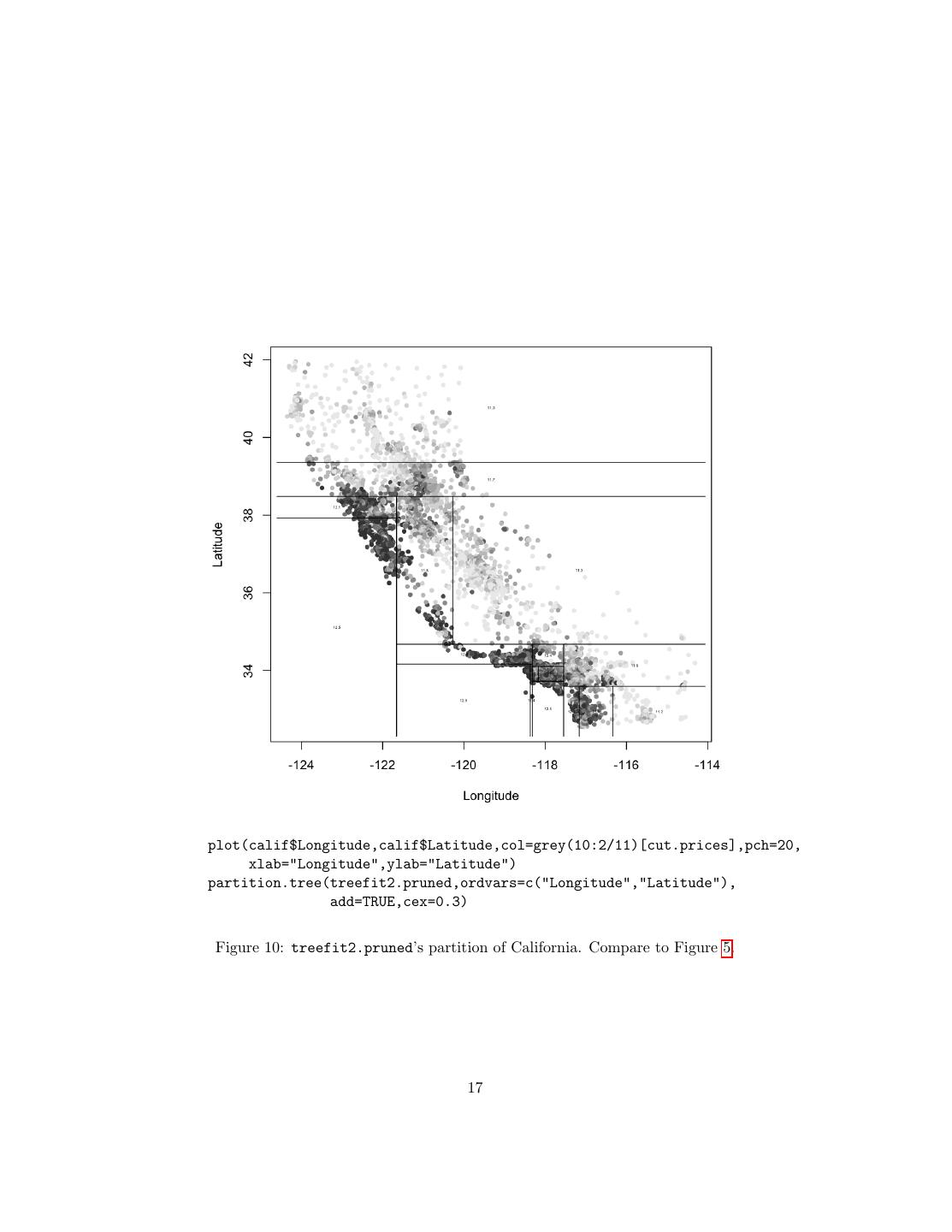
17 .plot(calif$Longitude,calif$Latitude,col=grey(10:2/11)[cut.prices],pch=20, xlab="Longitude",ylab="Latitude") partition.tree(treefit2.pruned,ordvars=c("Longitude","Latitude"), add=TRUE,cex=0.3) Figure 10: treefit2.pruned’s partition of California. Compare to Figure 5. 17 

18 .can separate the uncertainty in our predictions into two parts. First, we have some uncertainty in what our predictions should be, assuming the tree is correct. Second, we may of course be wrong about the tree. The first source of uncertainty — imprecise estimates of the conditional means within a given partition — is fairly easily dealt with. We can consis- tently estimate the standard error of the mean for leaf c as Vc /(nc − 1), just like we would for any other mean of IID samples. The second source is more troublesome; as the response values shift, the tree itself changes, and discontin- uously so, tree shape being a discrete variable. What we want is some estimate of how different the tree could have been, had we just drawn a different sample from the same source distribution. One way to estimate this, from the data at hand, is non-parametric boot- strapping. Given data (x1 , y1 ), (x2 , y2 ), . . . (xn , yn ), we draw a random set of integers J1 , J2 , . . . Jn , independently and uniformly from the numbers 1 : n, with replacement. Then we set (Xi , Yi ) = (xJi , yJi ) Each of the re-sample data points has the same distribution as the whole of the original data sample, and they’re independent. This is thus an IID sample of size n from the empirical distribution, and as close as we can get to another draw from the original data source without imposing any assumptions about how that’s distributed. We can now treat this bootstrap sample just like the original data and fit a tree to it. Repeated many times, we get a bootstrap sampling distribution of trees, which approximates the actual sampling distribution of regression trees. The spread of the predictions of our bootstrapped trees around that of our original gives us an indication of how our tree’s predictions are distributed around the truth. We will see more uses for bootstrapped trees next time, when we look at how to combine trees into forests. 3 Classification Trees Classification trees work just like regression trees, only they try to predict a dis- crete category (the class), rather than a numerical value. The variables which go into the classification — the inputs — can be numerical or categorical them- selves, the same way they can with a regression tree. They are useful for the same reasons regression trees are — they provide fairly comprehensible predic- tors in situations where there are many variables which interact in complicated, nonlinear ways. We find classification trees in almost the same way we found regression trees: we start with a single node, and then look for the binary distinction which gives us the most information about the class. We then take each of the resulting new nodes and repeat the process there, continuing the recursion until we reach some stopping criterion. The resulting tree will often be too large (i.e., over-fit), so 18 

19 .we prune it back using (say) cross-validation. The differences from regression- tree growing have to do with (1) how we measure information, (2) what kind of predictions the tree makes, and (3) how we measure predictive error. 3.1 Measuring Information The response variable Y is categorical, so we can use information theory to measure how much we learn about it from knowing the value of another discrete variable A: I[Y ; A] = Pr (A = a) I[Y ; A = a] (1) a where I[Y ; A = a] = H[Y ] − H[Y |A = a] (2) and you remember the definitions of entropy H[Y ] and conditional entropy H[Y |A = a]. I[Y ; A = a] is how much our uncertainty about Y decreases from knowing that A = a. (Less subjectively: how much less variable Y becomes when we go from the full population to the sub-population where A = a.) I[Y ; A] is how much our uncertainty about Y shrinks, on average, from knowing the value of A. For classification trees, A isn’t (necessarily) one of the predictors, but rather the answer to some question, generally binary, about one of the predictors X, i.e., A = 1A (X) for some set A. This doesn’t change any of the math above, however. So we chose the question in the first, root node of the tree so as to maximize I[Y ; A], which we calculate from the formula above, using the relative frequencies in our data to get the probabilities. When we want to get good questions at subsequent nodes, we have to take into account what we know already at each stage. Computationally, we do this by computing the probabilities and informations using only the cases in that node, rather than the complete data set. (Remember that we’re doing recursive partitioning, so at each stage the sub-problem looks just like a smaller version of the original problem.) Mathematically, what this means is that if we reach the node when A = a and B = b, we look for the question C which maximizes I[Y ; C|A = a, B = b], the information conditional on A = a, B = b. Algebraically, I[Y ; C|A = a, B = b] = H[Y |A = a, B = b] − H[Y |A = a, B = b, C] (3) Computationally, rather than looking at all the cases in our data set, we just look at the ones where A = a and B = b, and calculate as though that were all the data. Also, notice that the first term on the right-hand side, H[Y |A = a, B = b], does not depend on the next question C. So rather than maximizing I[Y ; C|A = a, B = b], we can just minimize H[Y |A = a, B = b, C]. 19 

20 .3.2 Making Predictions There are two kinds of predictions which a classification tree can make. One is a point prediction, a single guess as to the class or category: to say “this is a flower” or “this is a tiger” and nothing more. The other, a distributional prediction, gives a probability for each class. This is slightly more general, because if we need to extract a point prediction from a probability forecast we can always do so, but we can’t go in the other direction. For probability forecasts, each terminal node in the tree gives us a distribu- tion over the classes. If the terminal node corresponds to the sequence of answers A = a, B = b, . . . Q = q, then ideally this would give us Pr (Y = y|A = a, B = b, . . . Q = q) for each possible value y of the response. A simple way to get close to this is to use the empirical relative frequencies of the classes in that node. E.g., if there are 33 cases at a certain leaf, 22 of which are tigers and 11 of which are flowers, the leaf should predict “tiger with probability 2/3, flower with probability 1/3”. This is the maximum likelihood estimate of the true probability distribution, and we’ll write it Pr (·). Incidentally, while the empirical relative frequencies are consistent estimates of the true probabilities under many circumstances, nothing particularly com- pells us to use them. When the number of classes is large relative to the sample size, we may easily fail to see any samples at all of a particular class. The empirical relative frequency of that class is then zero. This is good if the actual probability is zero, not so good otherwise. (In fact, under the negative log- likelihood error discussed below, it’s infinitely bad, because we will eventually see that class, but our model will say it’s impossible.) The empirical relative frequency estimator is in a sense too reckless in following the data, without allowing for the possibility that it the data are wrong; it may under-smooth. Other probability estimators “shrink away” or “back off” from the empirical relative frequencies; Exercise 1 involves one such estimator. For point forecasts, the best strategy depends on the loss function. If it is just the mis-classification rate, then the best prediction at each leaf is the class with the highest conditional probability in that leaf. With other loss functions, we should make the guess which minimizes the expected loss. But this leads us to the topic of measuring error. 3.3 Measuring Error There are three common ways of measuring error for classification trees, or indeed other classification algorithms: misclassification rate, expected loss, and normalized negative log-likelihood, a.k.a. cross-entropy. 3.3.1 Misclassification Rate We’ve already seen this: it’s the fraction of cases assigned to the wrong class. 20 

21 .3.3.2 Average Loss The idea of the average loss is that some errors are more costly than others. For example, we might try classifying cells into “cancerous” or “not cancerous” based on their gene expression profiles6 . If we think a healthy cell from some- one’s biopsy is cancerous, we refer them for further tests, which are frightening and unpleasant, but not, as the saying goes, the end of the world. If we think a cancer cell is healthy, th consequences are much more serious! There will be a different cost for each combination of the real class and the guessed class; write Lij for the cost (“loss”) we incur by saying that the class is j when it’s really i. For an observation x, the classifier gives class probabilities Pr (Y = i|X = x). Then the expected cost of predicting j is: Loss(Y = j|X = x) = Lij Pr (Y = i|X = x) i A cost matrix might look as follows prediction truth “cancer” “healthy” “cancer” 0 100 “healthy” 1 0 We run an observation through the tree and wind up with class probabilities (0.4, 0.6). The most likely class is “healthy”, but it is not the most cost-effective decision. The expected cost of predicting “cancer” is 0.4 ∗ 0 + 0.6 ∗ 1 = 0.6, while the expected cost of predicting “healthy” is 0.4 ∗ 100 + 0.6 ∗ 0 = 40. The probability of Y = “healthy” must be 100 times higher than that of Y = “cancer” before “cancer” is a cost-effective prediction. Notice that if our estimate of the class probabilities is very bad, we can go through the math above correctly, but still come out with the wrong answer. If our estimates were exact, however, we’d always be doing as well as we could, given the data. You can show (and will, in the homework!) that if the costs are symmetric, we get the mis-classification rate back as our error function, and should always predict the most likely class. 3.3.3 Likelihood and Cross-Entropy The normalized negative log-likelihood is a way of looking not just at whether the model made the wrong call, but whether it made the wrong call with confi- dence or tentatively. (“Often wrong, never in doubt” is not a good idea.) More precisely, this loss function for a model Q is n 1 L(data, Q) = − log Q(Y = yi |X = xi ) n i=1 6 Think back to Homework 4, only there all the cells were cancerous, and the question was just “which cancer?” 21 

22 .where Q(Y = y|X = x) is the conditional probability the model predicts. If perfect classification were possible, i.e., if Y were a function of X, then the best classifier would give the actual value of Y a probability of 1, and L = 0. If there is some irreducible uncertainty in the classification, then the best possible classifier would give L = H[Y |X], the conditional entropy of Y given the inputs X. Less-than-ideal predictors have L > H[Y |X]. To see this, try re-write L so we sum over values rather than data-points: 1 L = − N (Y = y, X = x) log Q(Y = y|X = x) n x,y = − Pr (Y = y, X = x) log Q(Y = y|X = x) x,y = − Pr (X = x) Pr (Y = y|X = x) log Q(Y = y|X = x) x,y = − Pr (X = x) Pr (Y = y|X = x) log Q(Y = y|X = x) x y If the quantity in the log was Pr (Y = y|X = x), this would be H[Y |X]. Since it’s the model’s estimated probability, rather than the real probability, it turns out that this is always larger than the conditional entropy. L is also called the cross-entropy for this reason. There is a slightly subtle issue here about the difference between the in- sample loss, and the expected generalization error or risk. N (Y = y, X = x)/n = Pr (Y = y, X = x), the empirical relative frequency or empirical proba- bility. The law of large numbers says that this converges to the true probability, N (Y = y, X = x)/n → Pr (Y = y, X = x) as n → ∞. Consequently, the model which minimizes the cross-entropy in sample may not be the one which min- imizes it on future data, though the two ought to converge. Generally, the in-sample cross-entropy is lower than its expected value. Notice that to compare two models, or the same model on two different data sets, etc., we do not need to know the true conditional entropy H[Y |X]. All we need to know is that L is smaller the closer we get to the true class probabilities. If we could get L down to the cross-entropy, we would be exactly reproducing all the class probabilities, and then we could use our model to minimize any loss function we liked (as we saw above).7 7 Technically, if our model gets the class probabilities right, then the model’s predictions are just as informative as the original data. We then say that the predictions are a sufficient statistic for forecasting the class. In fact, if the model gets the exact probabilities wrong, but has the correct partition of the feature space, then its prediction is still a sufficient statistic. Under any loss function, the optimal strategy can be implemented using only a sufficient statistic, rather than needing the full, original data. This is an interesting but much more advanced topic; see, e.g., Blackwell and Girshick (1954) for details. 22 

23 .3.3.4 Neyman-Pearson Approach Using a loss function which assigns different weights to different error types has two noticeable drawbacks. First of all, we have to pick the weights, and this is often quite hard to do. Second, whether our classifier will do well in the future depends on getting the same proportion of cases in the future. Suppose that we’re developing a tree to classify cells as cancerous or not from their gene expression profiles8 . We will probably want to include lots of cancer cells in our training data, so that we can get a good idea of what cancers look like, biochemically. But, fortunately, most cells are not cancerous, so if doctors start applying our test to their patients, they’re going to find that it massively over-diagnoses cancer — it’s been calibrated to a sample where the proportion (cancer):(healthy) is, say, 1:1, rather than, say, 1:20.9 There is an alternative to weighting which deals with both of these issues, and deserves to be better known and more widely-used than it is. This was introduced by Scott and Nowak (2005), under the name of the “Neyman-Pearson approach” to statistical learning. The reasoning goes as follows. When we do a binary classification problem, we’re really doing a hypothesis test, and the central issue in hypothesis testing, as first recognized by Neyman and Pearson, is to distinguish between the rates of different kinds of errors: false positives and false negatives, false alarms and misses, type I and type II. The Neyman-Pearson approach to designing a hypothesis test is to first fix a limit on the false positive probability, the size of the test, canonically α. Then, among all tests of size α, we want to minimize the false negative rate, or equivalently maximize the power, β. In the traditional theory of testing, we know the distribution of the data under the null and alternative hypotheses, and so can (in principle) calculate α and β for any given test. This is not the case in data mining, but we do generally have very large samples generated under both distributions (depending on the class of the data point). If we fix α, we can ask, for any classifier — say, a tree — whether its false alarm rate is ≤ α. If so, we keep it for further consideration; if not, we discard it. Among those with acceptable false alarm rates, then, we ask “which classifier has the lowest false negative rate, the highest β?” This is the one we select. Notice that this solves both problems with weighting. We don’t have to pick a weight for the two errors; we just have to say what rate of false positives α we’re willing to accept. There are many situations where this will be easier to do than to fix on a relative cost. Second, the rates α and β are properties of the conditional distributions of the features, Pr (X|Y ). If those conditional distributions stay they same but the proportions of the classes change, then the error rates are unaffected. Thus, training the classifier with a different mix of cases than we’ll encounter in the future is not an issue. 8 This is almost like homework 4, except there all the cells were from cancers of one sort or another. 9 Cancer is rarer than that, but realistically doctors aren’t going to run a test like this unless they have some reason to suspect cancer might be present. 23 

24 . Unfortunately, I don’t know of any R implementation of Neyman-Pearson learning; it wouldn’t be hard, I think, but goes beyond one problem set at this level. 4 Further Reading The classic book on prediction trees, which basically introduced them into statis- tics and data mining, is Breiman et al. (1984). Chapter three in Berk (2008) is clear, easy to follow, and draws heavily on Breiman et al. Another very good chapter is the one on trees in Ripley (1996), which is especially useful for us because Ripley wrote the tree package. (The whole book is strongly recom- mended if you plan to go further in data-mining.) There is another tradition of trying to learn tree-structured models which comes out of artificial intelligence and inductive logic; see Mitchell (1997). The clearest explanation of the Neyman-Pearson approach to hypothesis testing I have ever read is that in Reid (1982), which is one of the books which made me decide to learn statistics. 5 Exercises To think through, not to hand in. k 1. Suppose that we see each of k classes ni times, with i=1 ni = n. The maximum likelihood estimate of the probability of the ith class is pi = ni /n. Suppose that instead we use the estimates ni + 1 p˜i = k (4) j=1 nj + 1 This estimator goes back to Laplace, who called it the “rule of succession”. Show that the p˜i sum up to one. Show, using the law of large numbers, that p˜ → p when p → p. Do these properties still hold if the +1s in the numerator and denominator are replaced by +d for an arbitrary d > 0? 2. Fun with Laplace’s rule of succession: will the Sun rise tomorrow? One illustration Laplace gave of this probability estimator was the following. Suppose we know, from written records, that the Sun has risen in the east every day for the last 4000 years.10 (a) Calculate the probability of the event “the Sun will rise in the east tomorrow”, using Eq. 4. You may take the year as containing 365.256 days. 10 Laplace was thus ignoring people who live above the Artic circle, or below the Antarctic circle. The latter seems particularly unfair, because so many of them are scientists. 24 

25 . (b) Calculate the probability that the Sun will rise in the east every day for the next four thousand years, assuming this is an IID event. Is this a reasonable assumption? (c) Calculate the probability of the event “the Sun will rise in the east every day for four thousand years” directly from Eq. 4. Does your answer agree with part (b)? Should it? Laplace did not, of course, base his belief that the Sun will rise in the morning on such calculations; besides everything else, he was the world’s expert in celestial mechanics! But this shows the problem with the 3. Show that, when all the off-diagonal elements of Lij are equal (and posi- tive!), the best class to predict is always the most probable class. References Berk, Richard A. (2008). Statistical Learning from a Regression Perspective. Springer Series in Statistics. New York: Springer-Verlag. Blackwell, David and M. A. Girshick (1954). Theory of Games and Statistical Decisions. New York: Wiley. Breiman, Leo, Jerome Friedman, R. Olshen and C. Stone (1984). Classification and Regression Trees. Belmont, California: Wadsworth. Mitchell, Tom M. (1997). Machine Learning. New York: McGraw-Hill. Reid, Constance (1982). Neyman from Life. New York: Springer-Verlag. Ripley, Brian D. (1996). Pattern Recognition and Neural Networks. Cambridge, England: Cambridge University Press. Scott, C. and R. Nowak (2005). “A Neyman-Pearson Approach to Statisti- cal Learning.” IEEE Transactions on Information Theory, 51: 3806–3819. doi:10.1109/TIT.2005.856955. 25