MRF和分割与图形切割

1 .Markov Random Fields and Segmentation with Graph Cuts Computer Vision Jia-Bin Huang, Virginia Tech Many slides from D. Hoiem

2 .Administrative stuffs Final project Proposal due Oct 27 (Thursday ) HW 4 is out Due 11:59pm on Wed, November 2nd, 2016

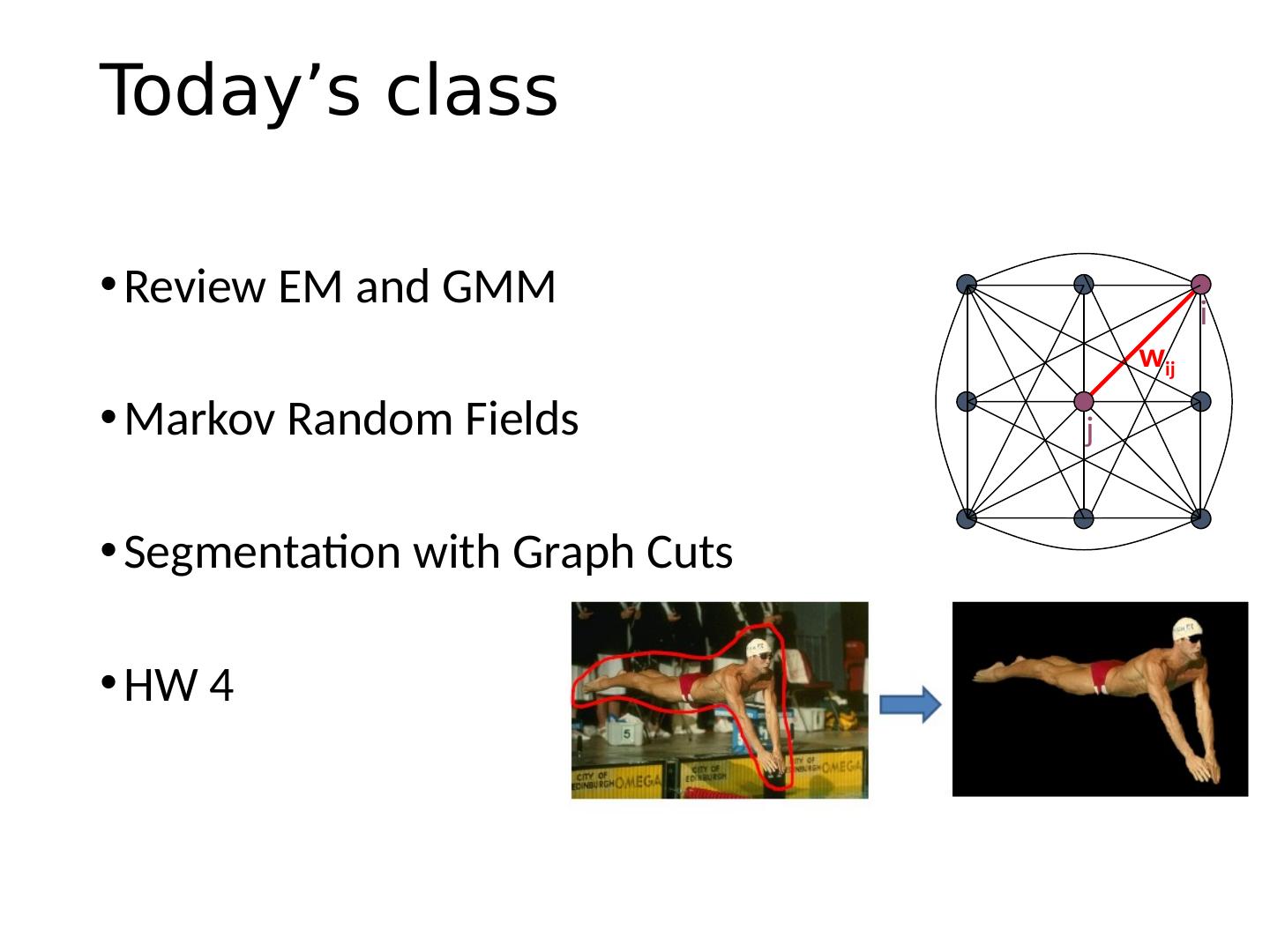
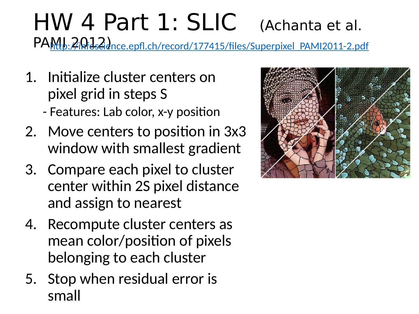
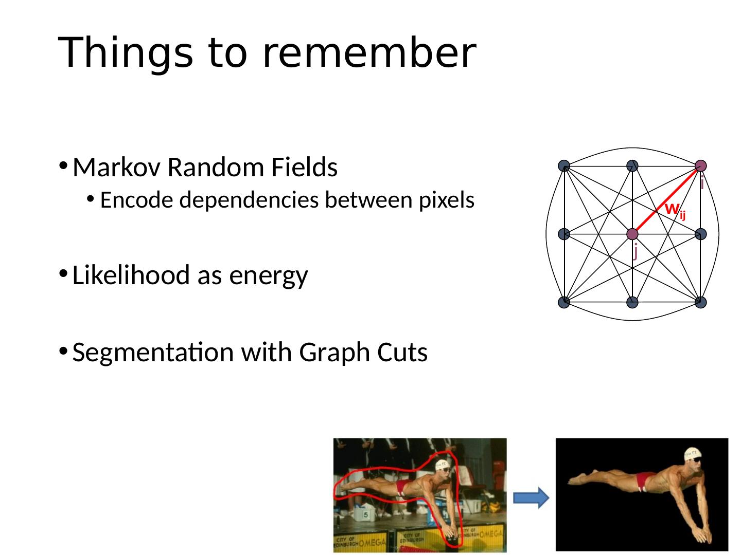
3 .Today’s class Review EM and GMM Markov Random Fields Segmentation with Graph Cuts HW 4 i j w ij

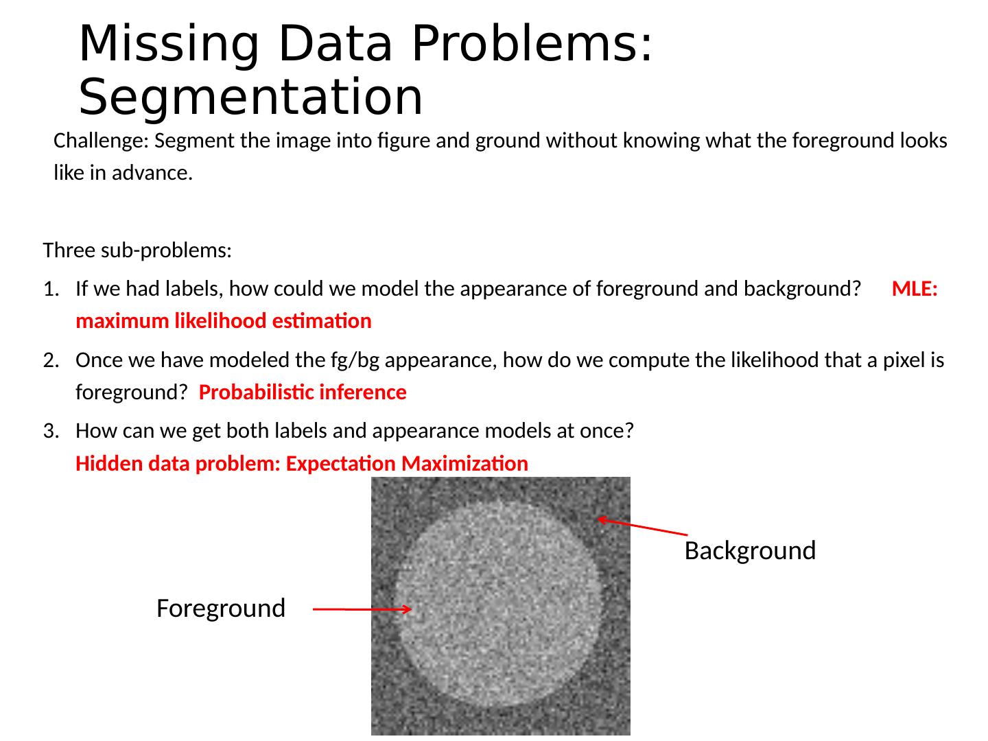
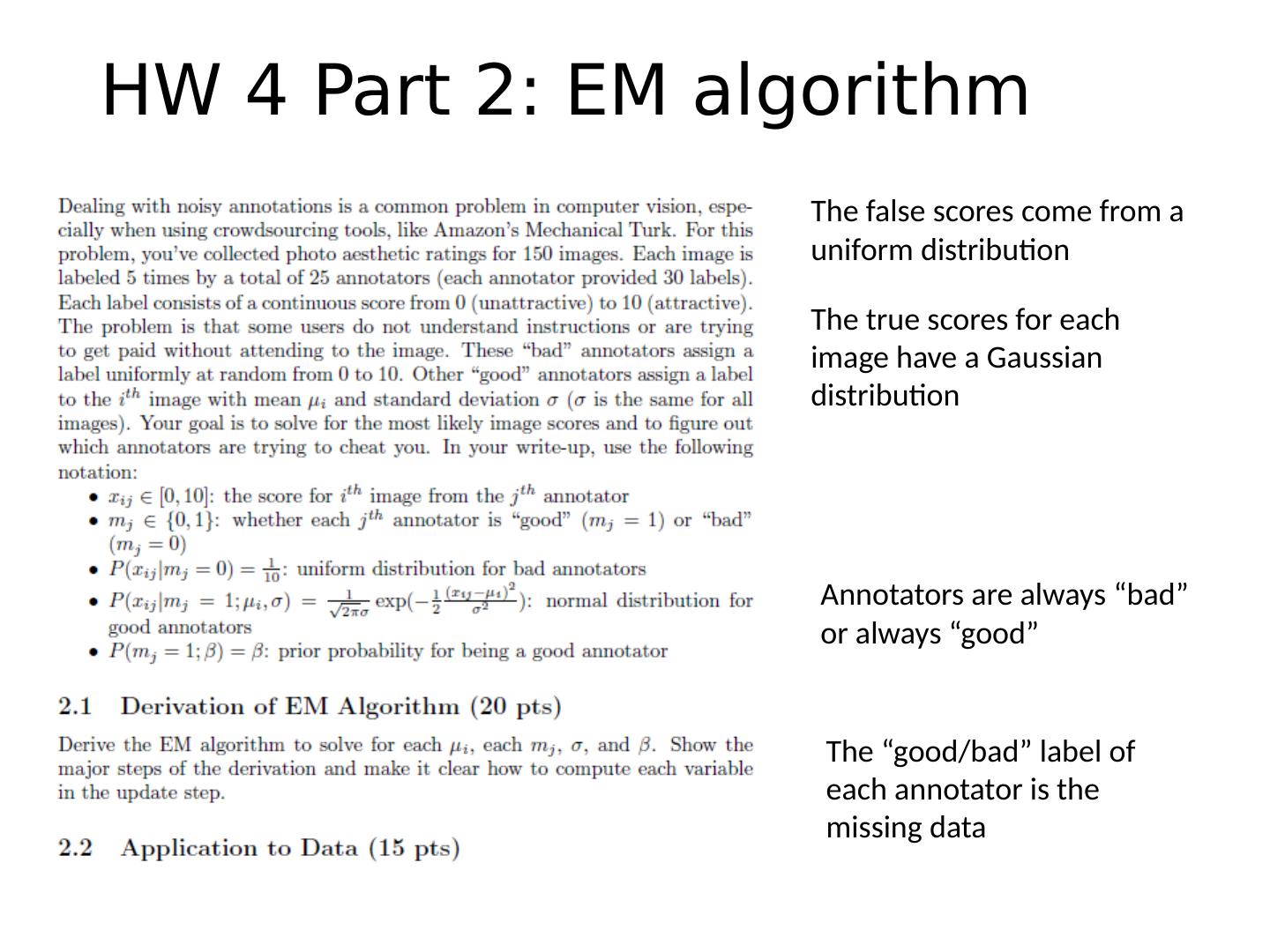
4 .Missing Data Problems: Segmentation Challenge: Segment the image into figure and ground without knowing what the foreground looks like in advance. Three sub-problems: If we had labels, how could we model the appearance of foreground and background? MLE: maximum likelihood estimation Once we have modeled the fg / bg appearance, how do we compute the likelihood that a pixel is foreground? Probabilistic inference How can we get both labels and appearance models at once? Hidden data problem: Expectation Maximization Foreground Background

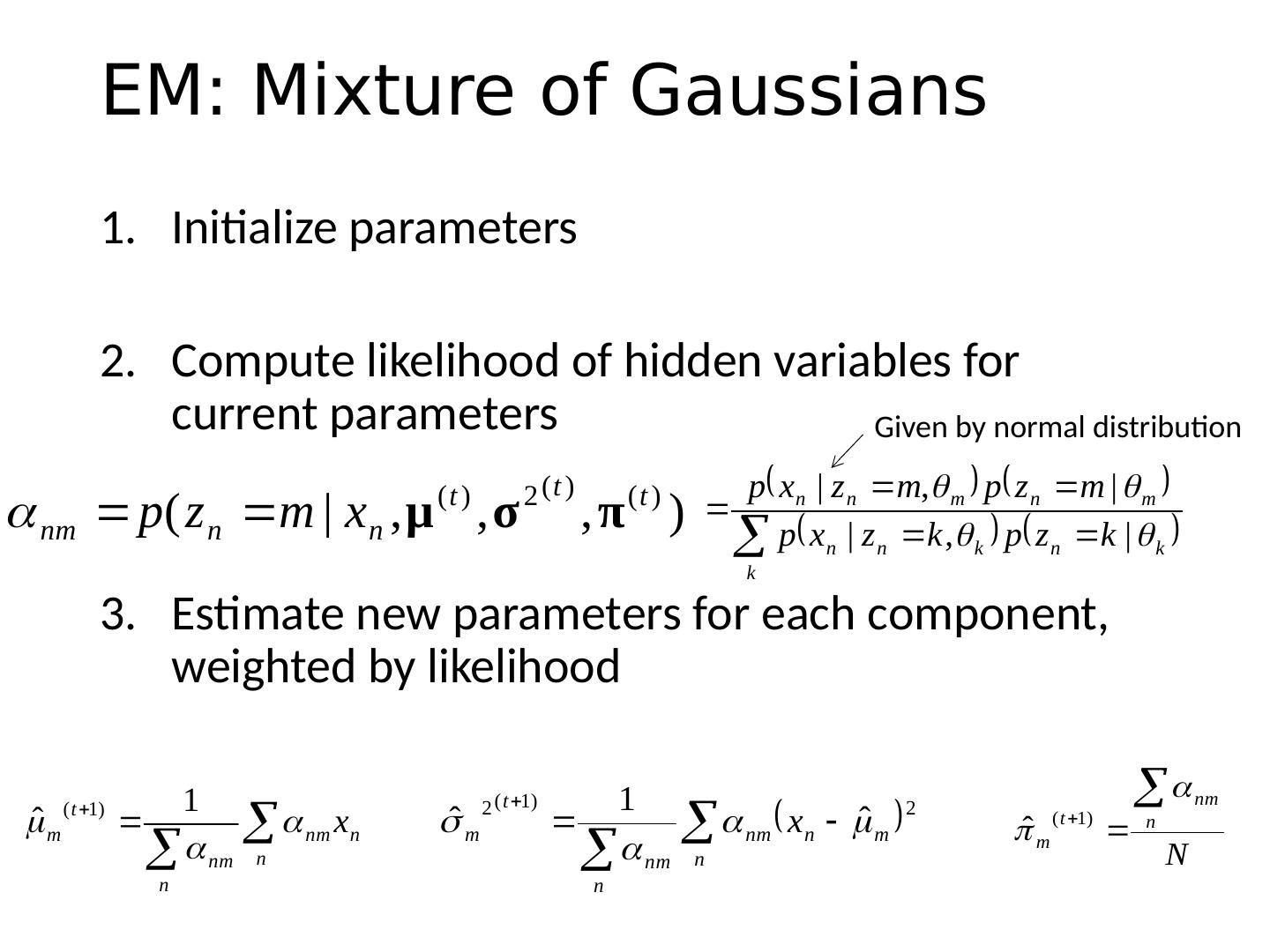
5 .EM: Mixture of Gaussians Initialize parameters Compute likelihood of hidden variables for current parameters Estimate new parameters for each component, weighted by likelihood Given by normal distribution

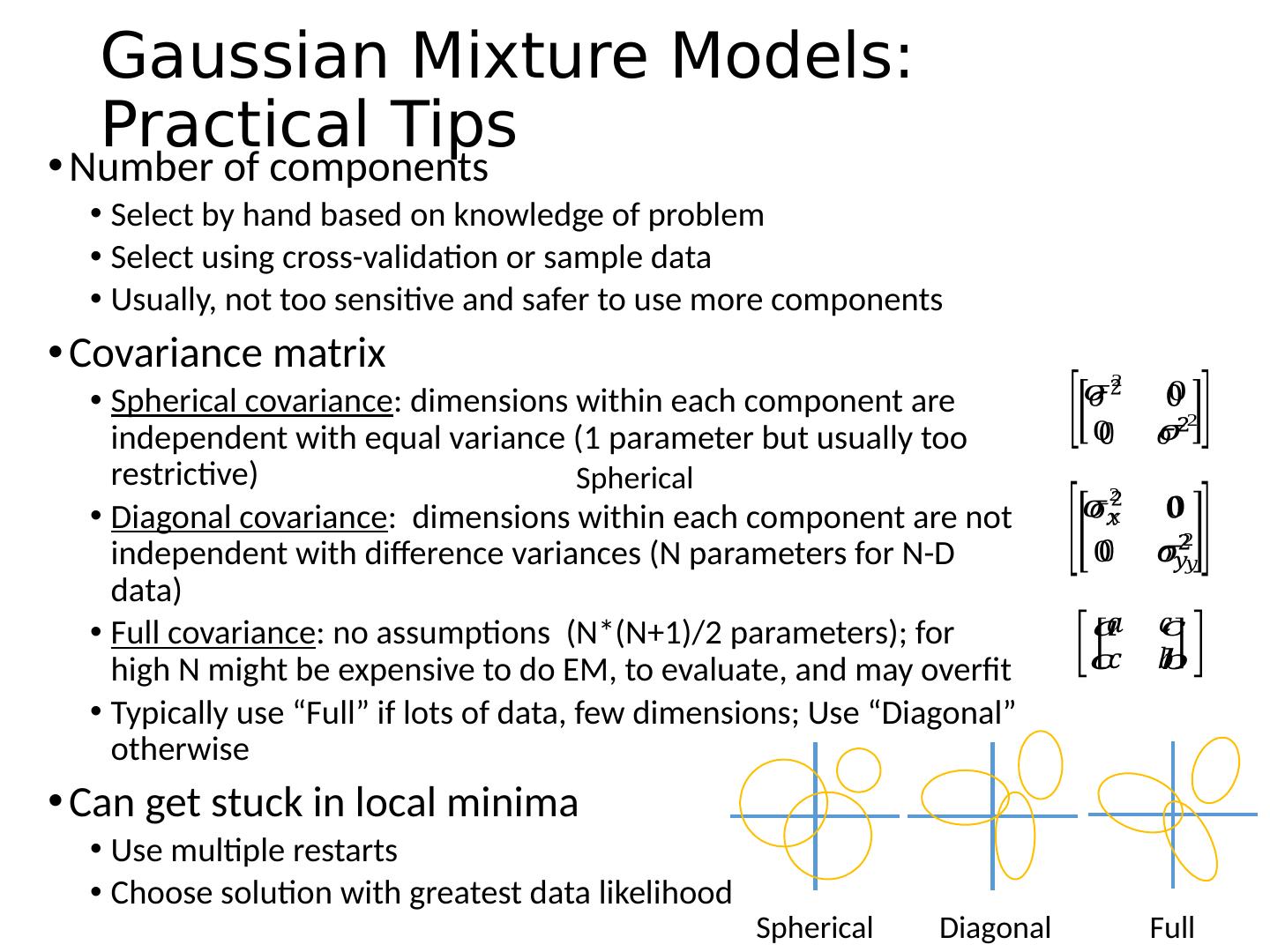
6 .Gaussian Mixture M odels: Practical Tips Number of components Select by hand based on knowledge of problem Select using cross-validation or sample data Usually , not too sensitive and safer to use more components Covariance matrix Spherical covariance : dimensions within each component are independent with equal variance (1 parameter but usually too restrictive) Diagonal covariance : dimensions within each component are not independent with difference variances (N parameters for N-D data) Full covariance : no assumptions (N*(N+1)/2 parameters); for high N might be expensive to do EM, to evaluate, and may overfit Typically use “Full” if lots of data, few dimensions; Use “Diagonal” otherwise Can get stuck in local minima Use multiple restarts Choose solution with greatest data likelihood       Spherical Spherical Diagonal Full

7 .“Hard EM” Same as EM except compute z* as most likely values for hidden variables K-means is an example Advantages Simpler: can be applied when cannot derive EM Sometimes works better if you want to make hard predictions at the end But Generally, pdf parameters are not as accurate as EM

8 .EM Demo GMM with images demos

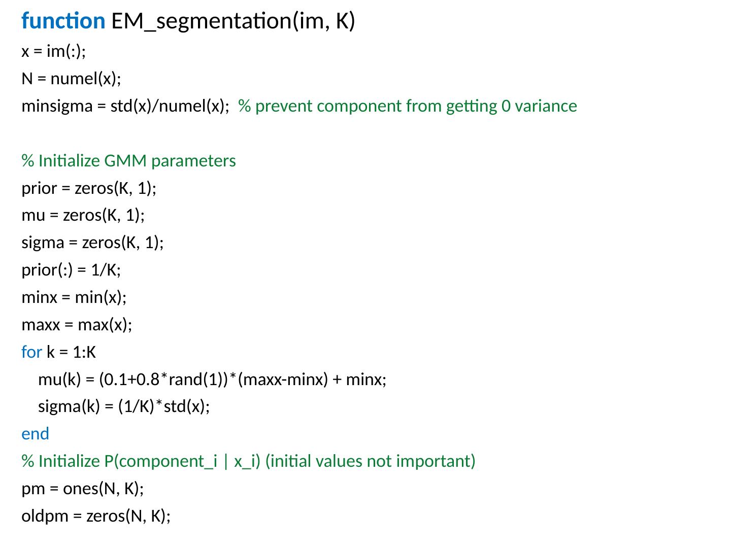
9 .function EM_segmentation ( im , K) x = im (:); N = numel (x); minsigma = std (x)/ numel (x); % prevent component from getting 0 variance % Initialize GMM parameters prior = zeros(K, 1); mu = zeros(K, 1); sigma = zeros(K, 1); prior(:) = 1/K; minx = min(x); maxx = max(x); for k = 1:K mu(k) = (0.1+0.8*rand(1))*( maxx -minx) + minx; sigma(k) = (1/K)* std (x); end % Initialize P( component_i | x_i ) (initial values not important) pm = ones(N, K); oldpm = zeros(N, K);

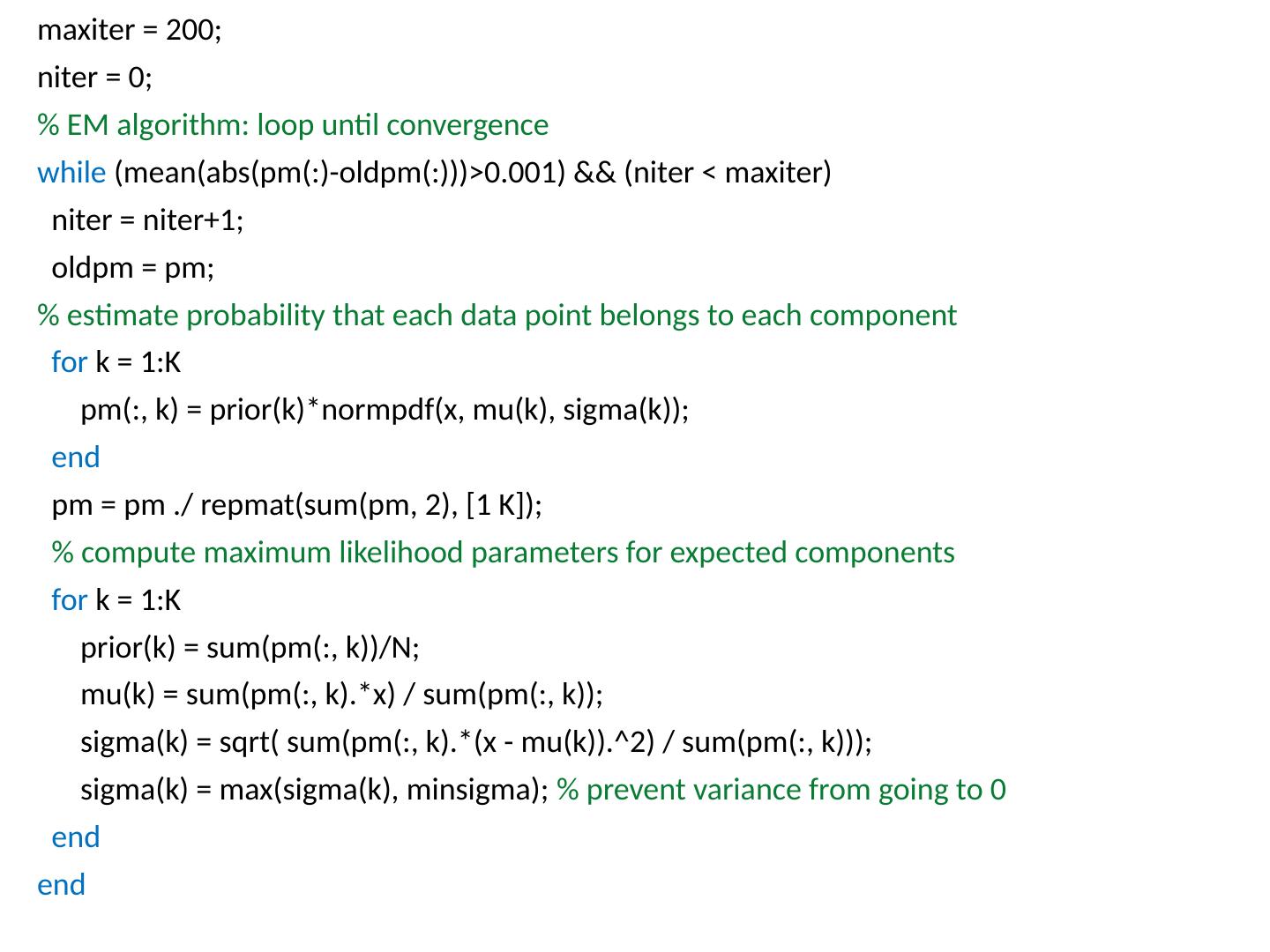
10 .maxiter = 200; niter = 0 ; % EM algorithm: loop until convergence while (mean(abs(pm(:)- oldpm (:)))>0.001) && (niter < maxiter ) niter = niter+1; oldpm = pm; % estimate probability that each data point belongs to each component for k = 1:K pm(:, k) = prior(k)* normpdf (x, mu(k), sigma(k)); end pm = pm ./ repmat (sum(pm, 2), [1 K ]); % compute maximum likelihood parameters for expected components for k = 1:K prior(k) = sum(pm(:, k))/N; mu(k) = sum(pm(:, k).*x) / sum(pm(:, k)); sigma(k) = sqrt ( sum(pm(:, k).*(x - mu(k)).^2) / sum(pm(:, k))); sigma(k) = max(sigma(k), minsigma ); % prevent variance from going to 0 end end

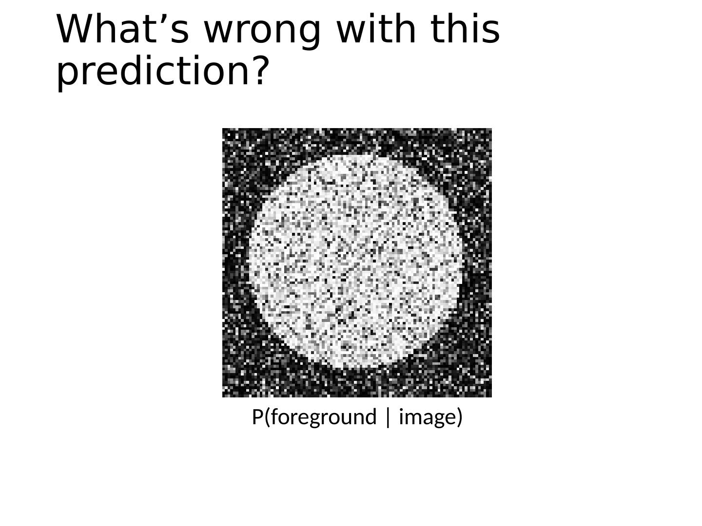
11 .What’s wrong with this prediction? P(foreground | image)

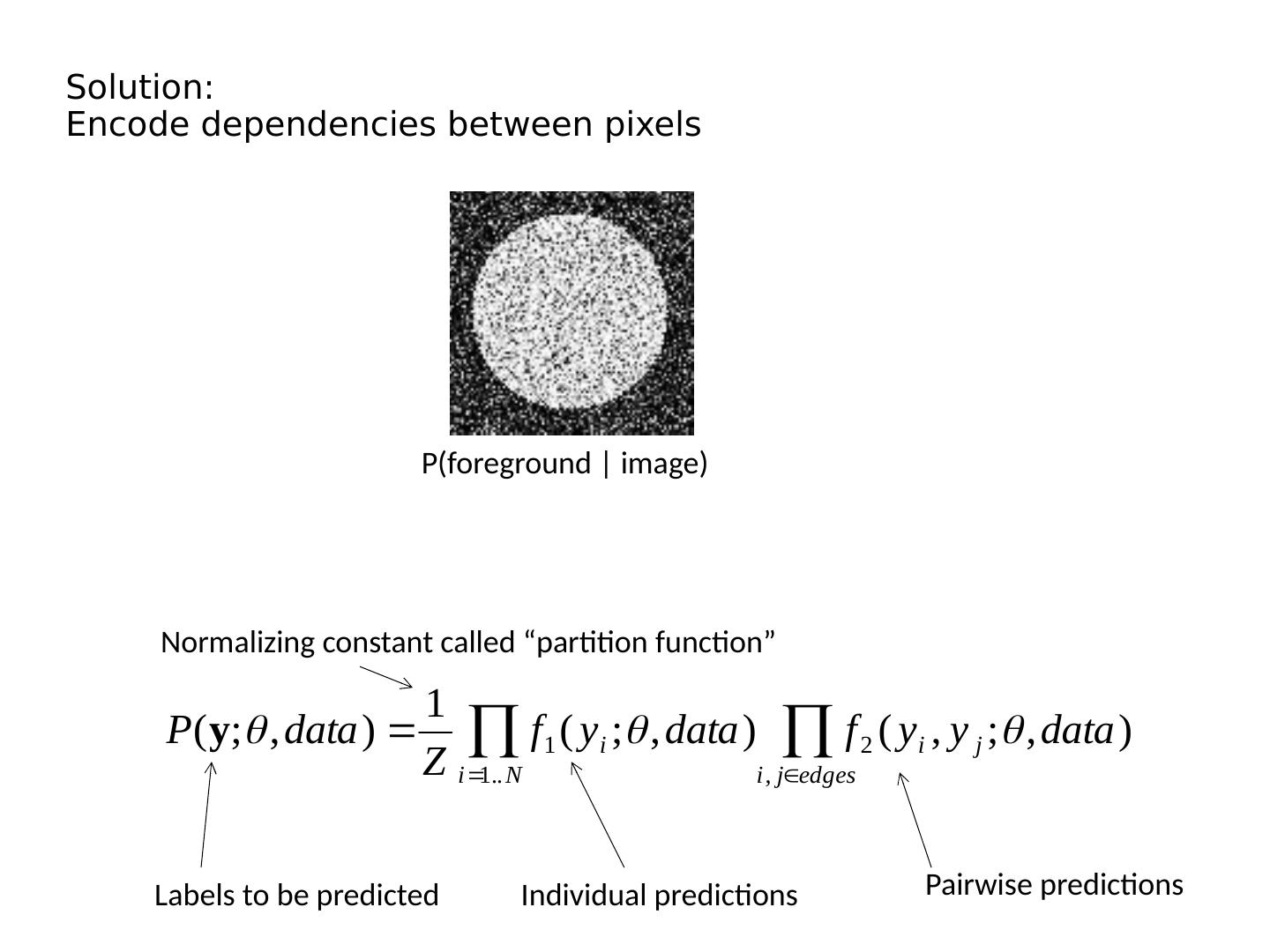
12 .Solution: Encode dependencies between pixels P(foreground | image) Labels to be predicted Individual predictions Pairwise predictions Normalizing constant called “partition function”

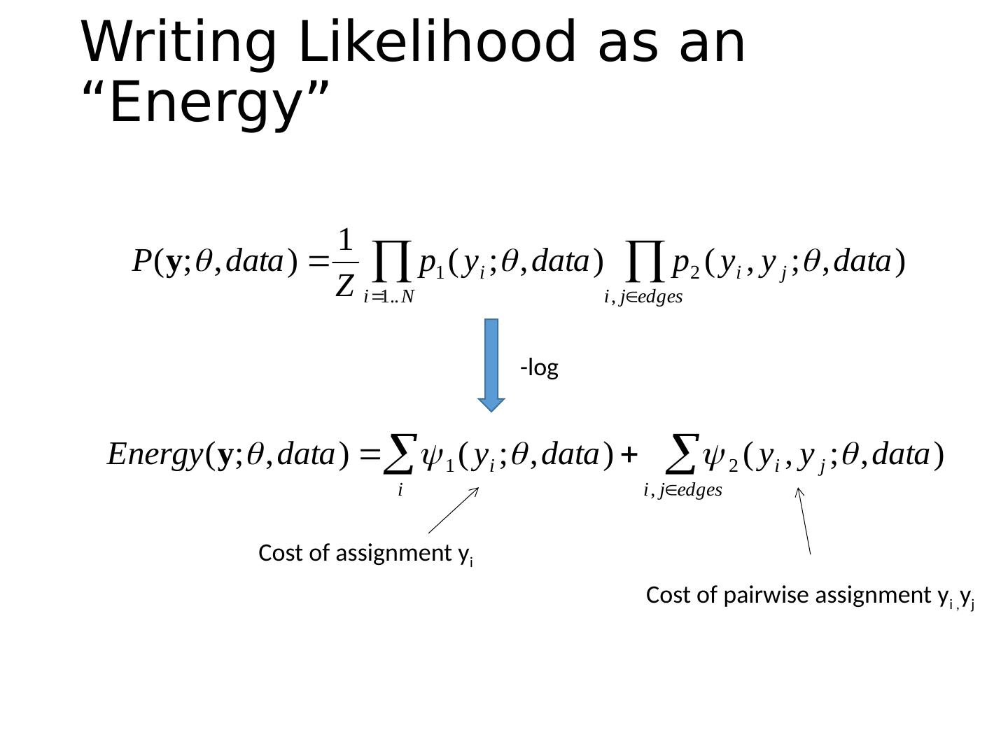
13 .Writing Likelihood as an “Energy” Cost of assignment y i Cost of pairwise assignment y i , y j -log

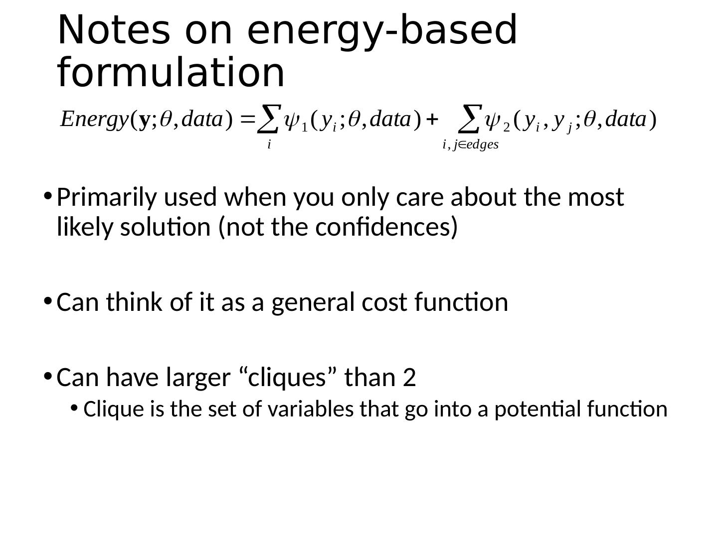
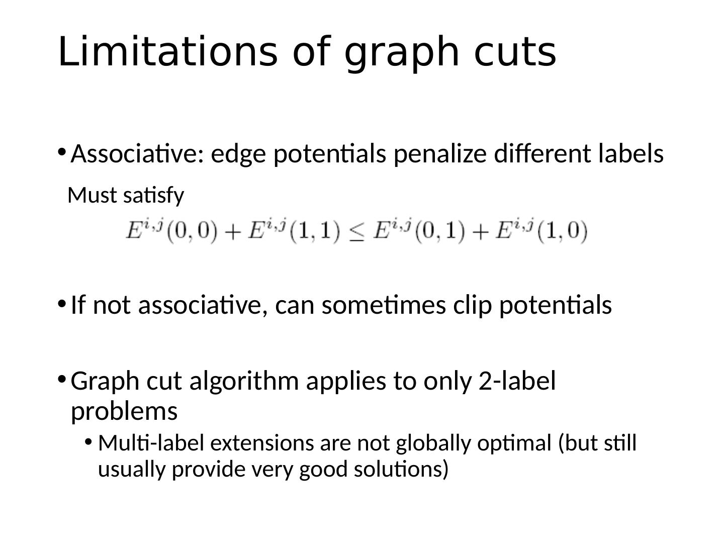
14 .Notes on energy-based formulation Primarily used when you only care about the most likely solution (not the confidences) Can think of it as a general cost function Can have larger “cliques” than 2 Clique is the set of variables that go into a potential function

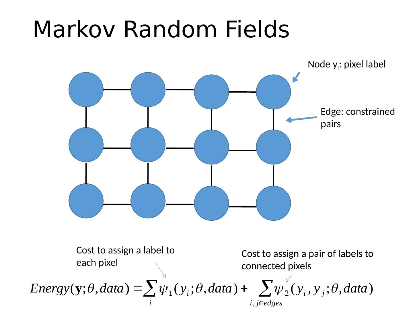
15 .Markov Random Fields Node y i : pixel label Edge: constrained pairs Cost to assign a label to each pixel Cost to assign a pair of labels to connected pixels

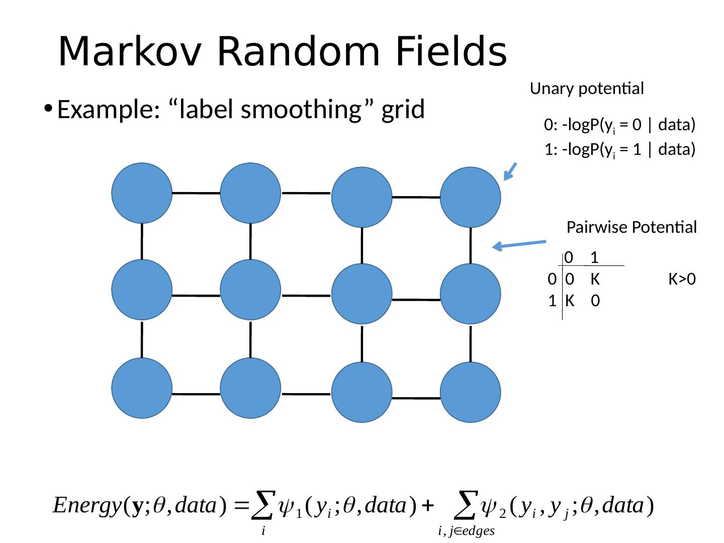
16 .Markov Random Fields Example: “label smoothing” grid Unary potential 0 1 0 0 K 1 K 0 Pairwise Potential 0: - logP ( y i = 0 | data) 1 : - logP ( y i = 1 | data) K>0

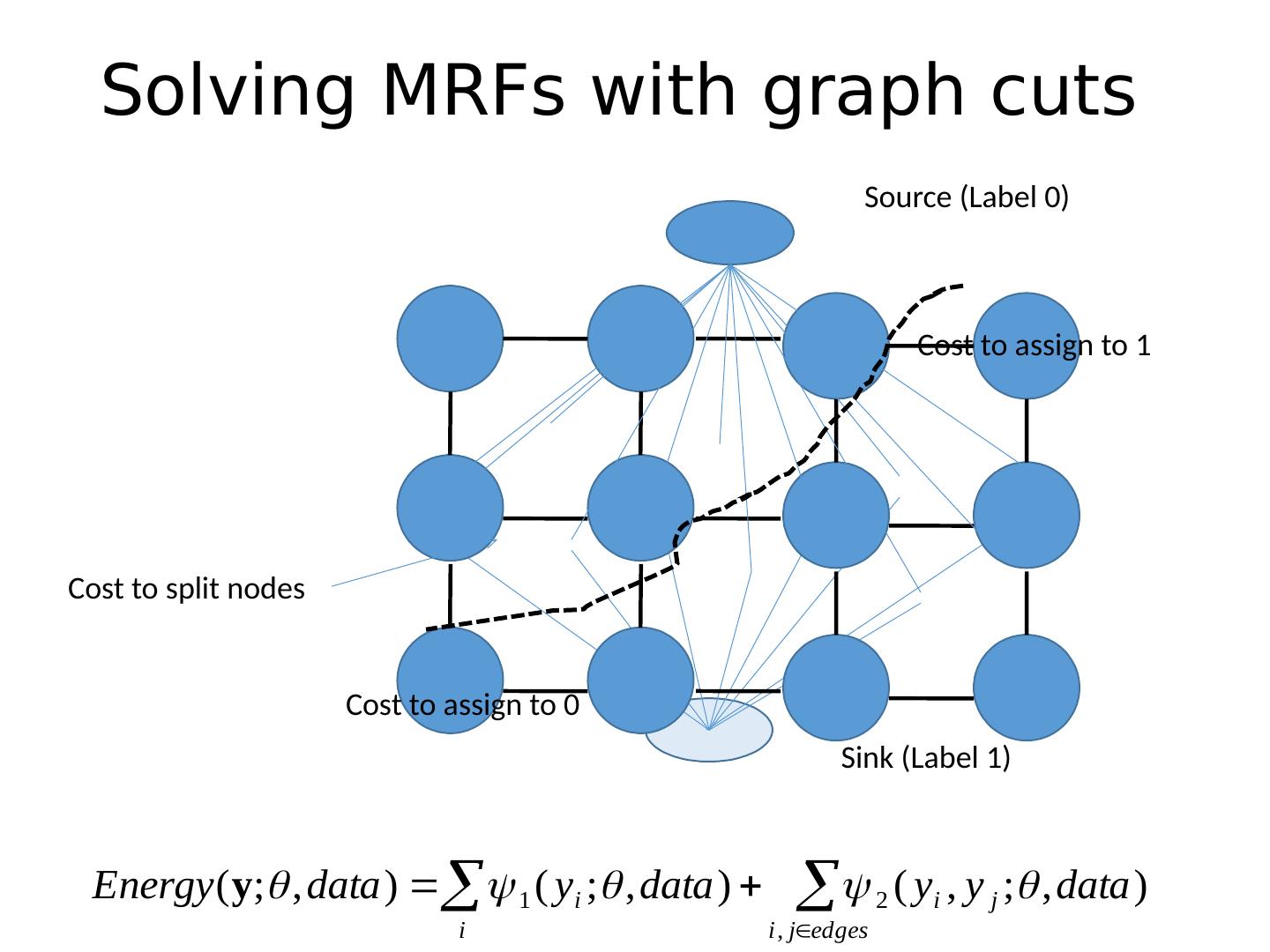
17 .Solving MRFs with graph cuts Source (Label 0) Sink (Label 1) Cost to assign to 1 Cost to assign to 0 Cost to split nodes

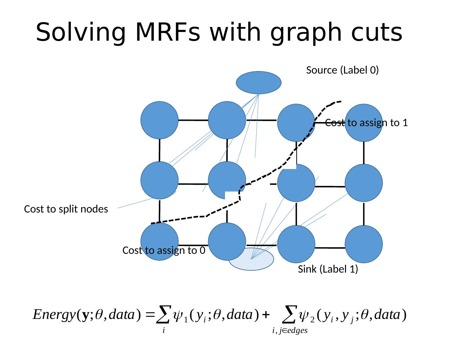
18 .Solving MRFs with graph cuts Source (Label 0) Sink (Label 1) Cost to assign to 1 Cost to assign to 0 Cost to split nodes

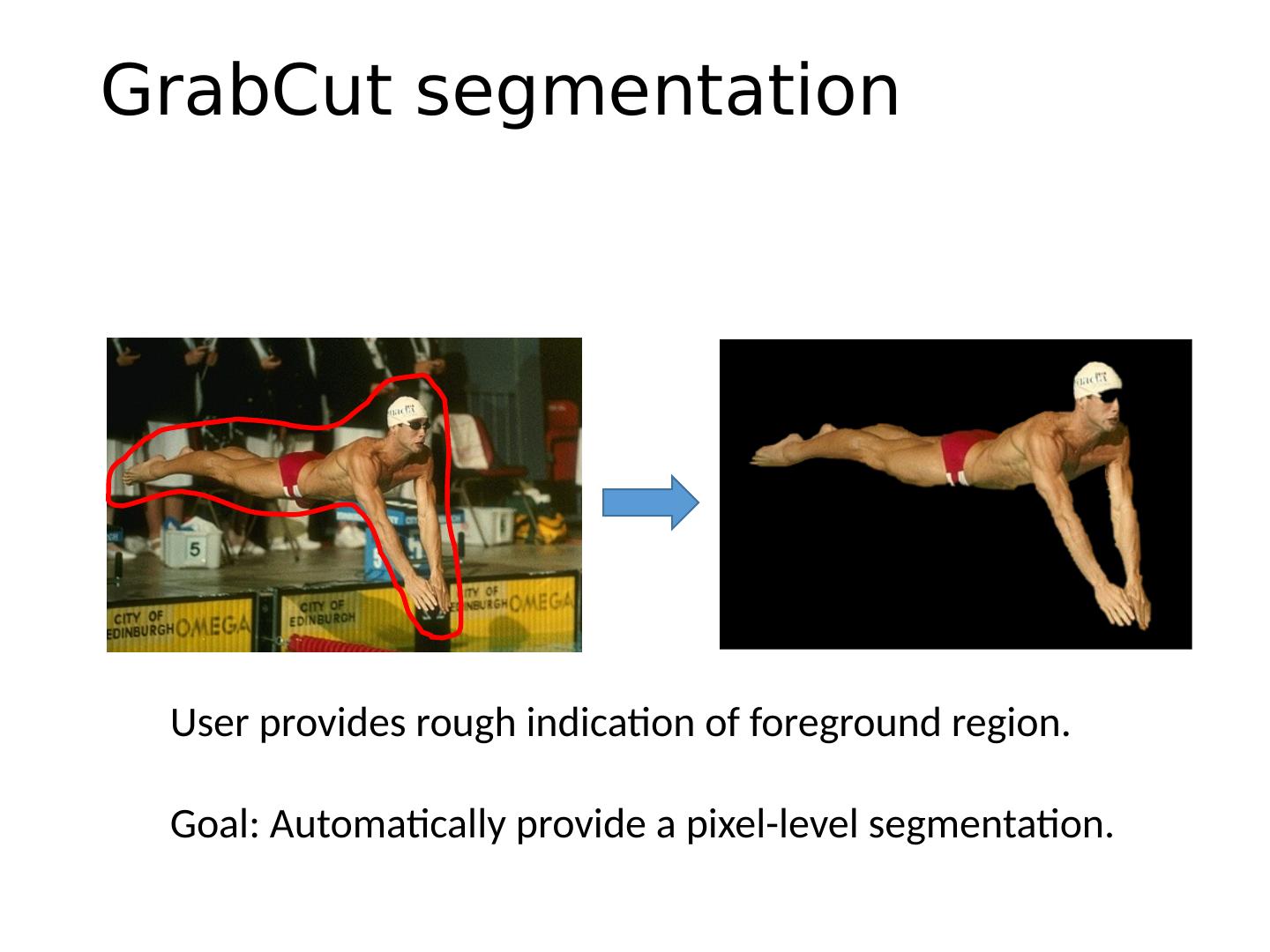
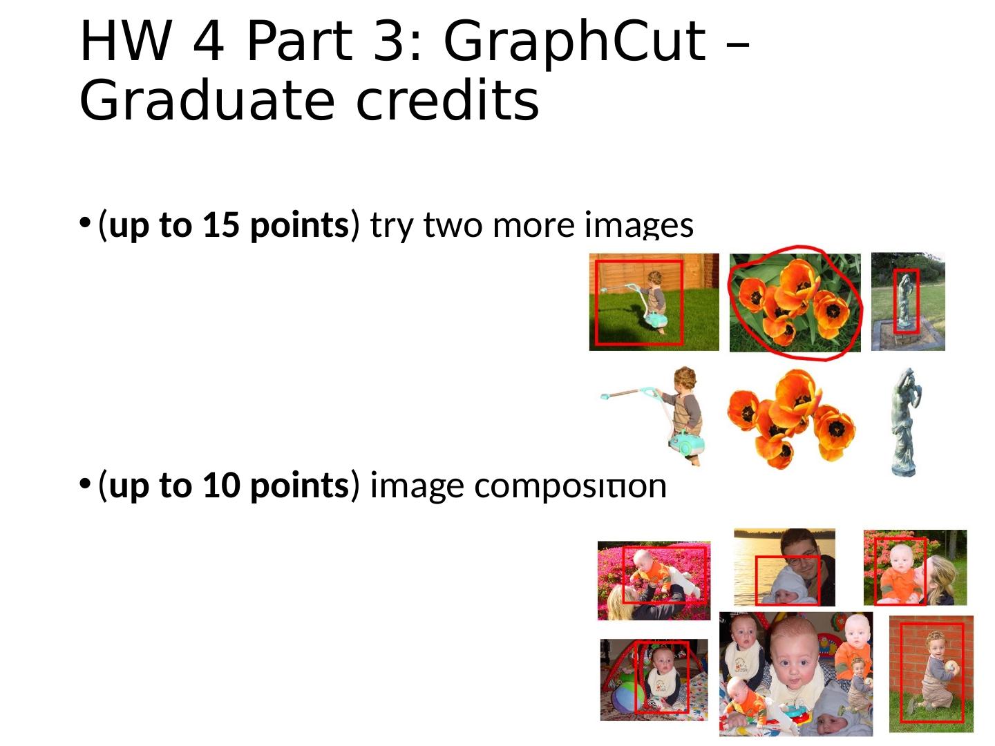
19 .GrabCut segmentation User provides rough indication of foreground region. Goal: Automatically provide a pixel-level segmentation.

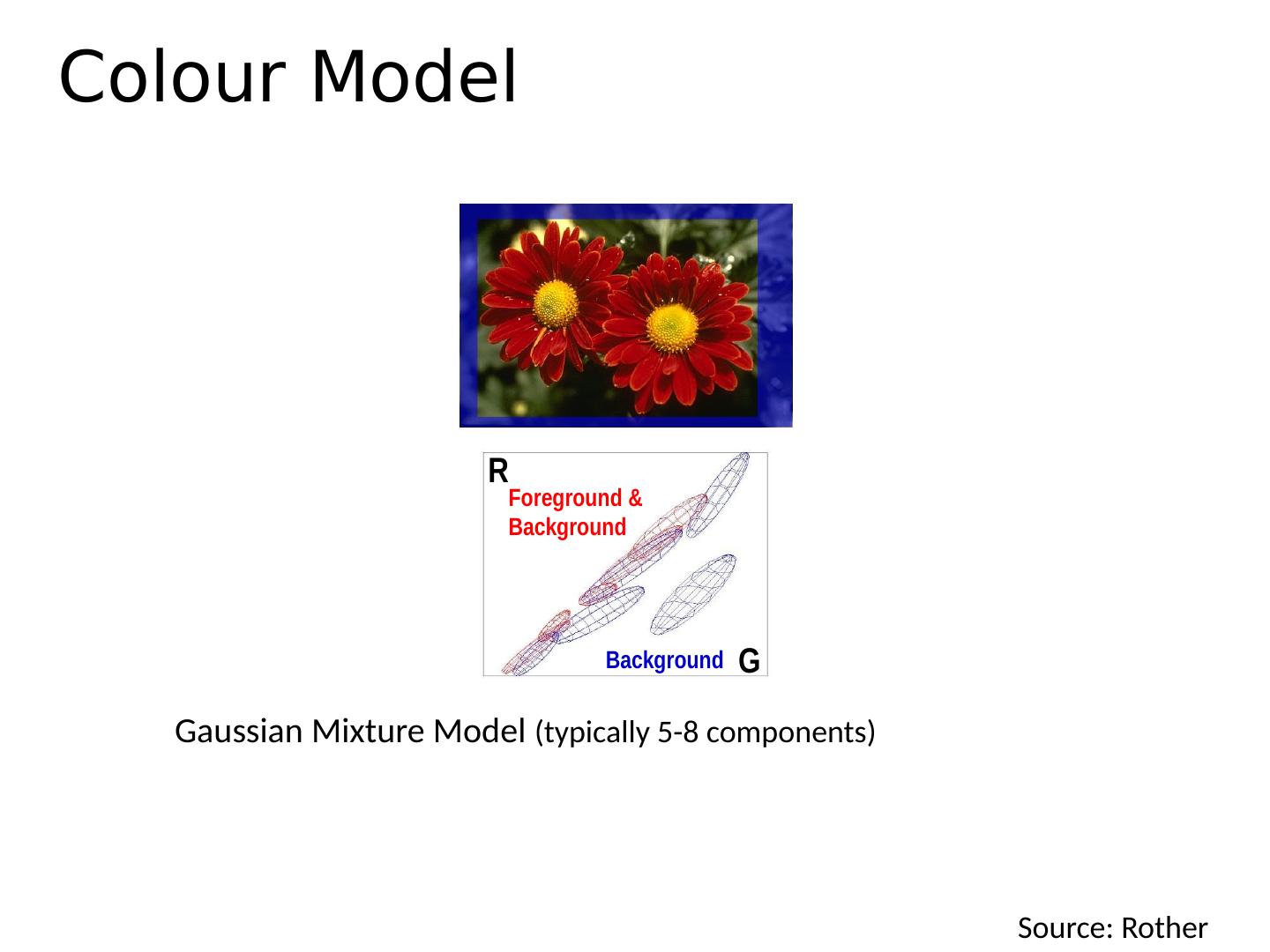
20 . Colour Model Gaussian Mixture Model (typically 5-8 components) Foreground & Background Background G R Source: Rother

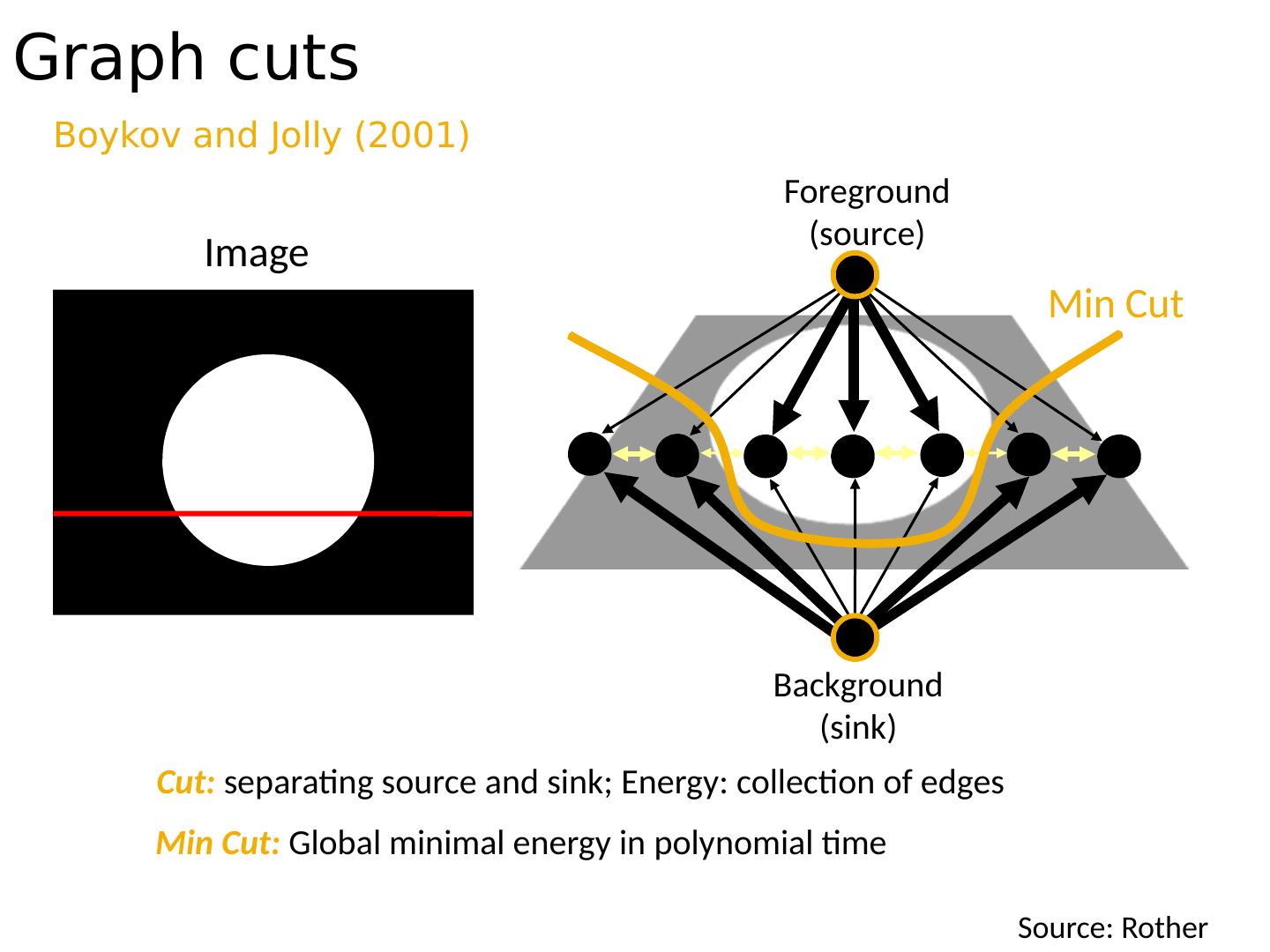
21 .Graph cuts Boykov and Jolly (2001) Image Min Cut Cut: separating source and sink; Energy: collection of edges Min Cut: Global minimal energy in polynomial time Foreground (source) Background (sink) Source: Rother

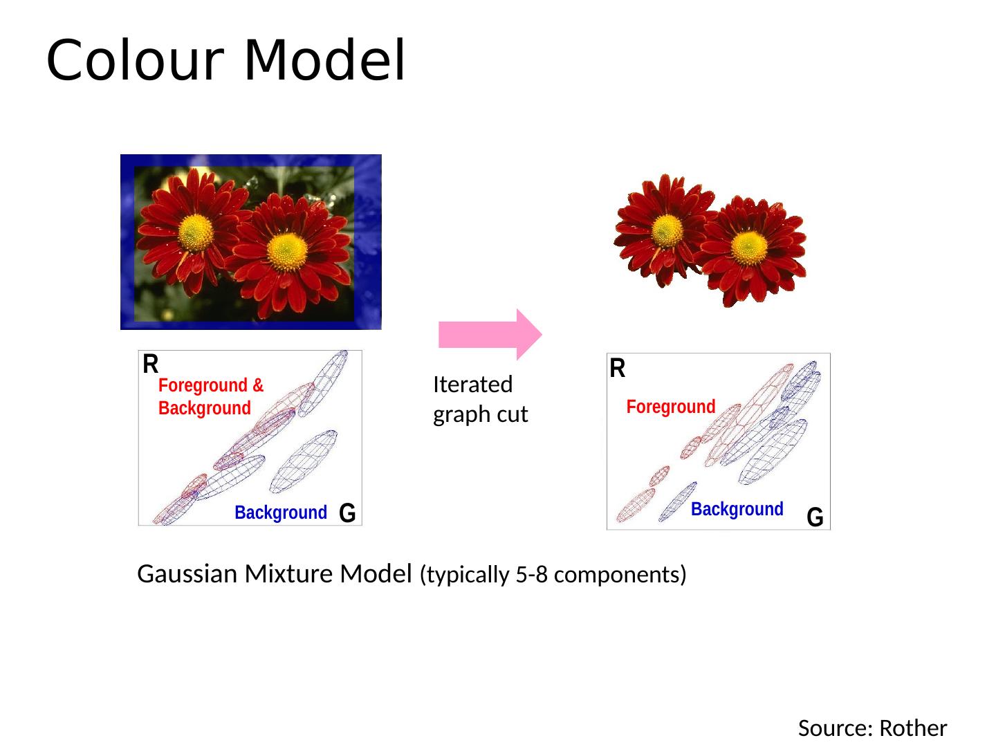
22 . Colour Model Gaussian Mixture Model (typically 5-8 components) Foreground & Background Background Foreground Background G R G R Iterated graph cut Source: Rother

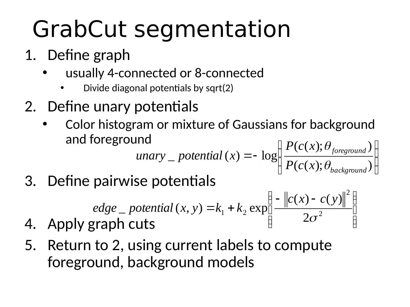
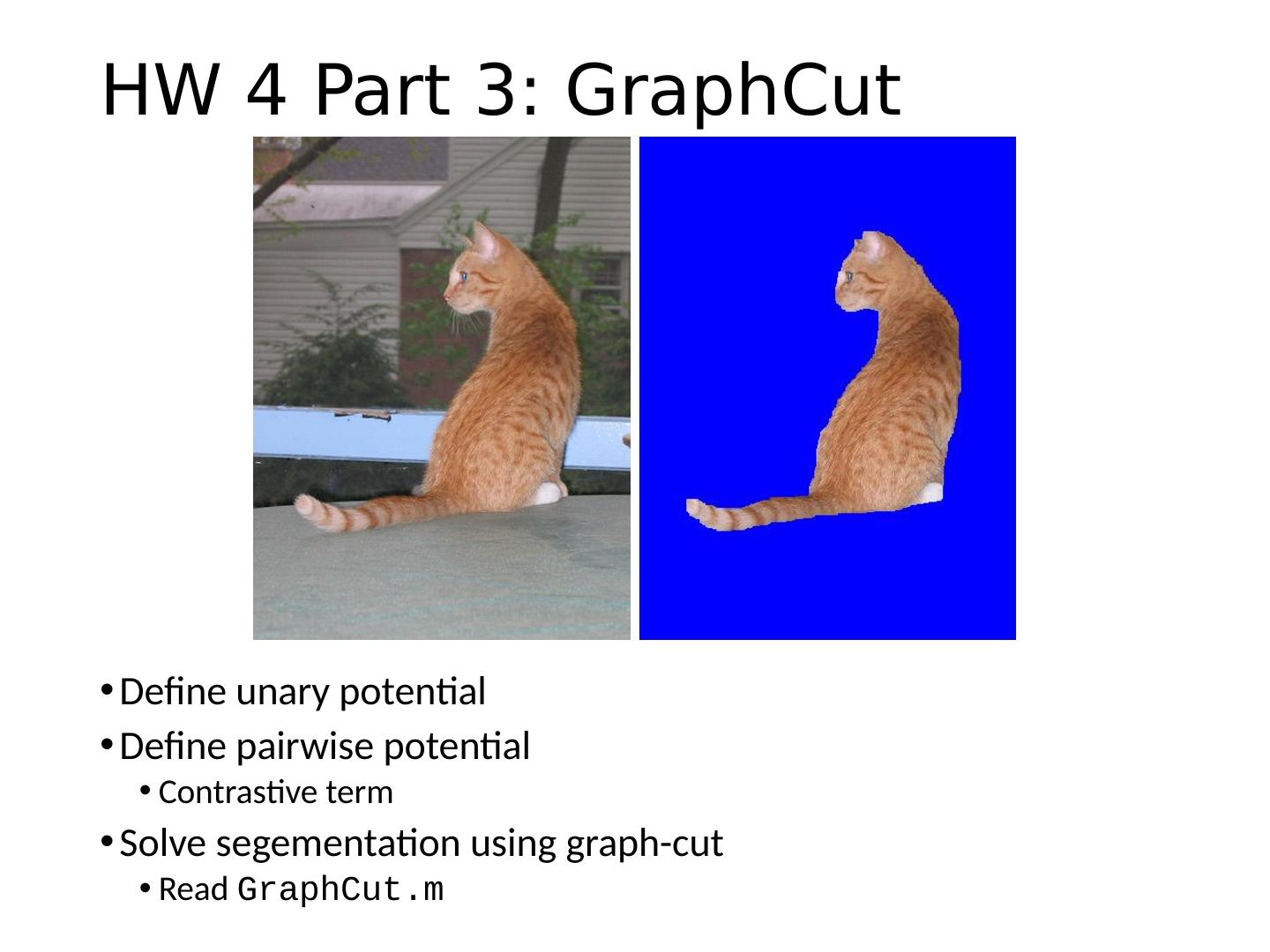
23 .GrabCut segmentation Define graph usually 4-connected or 8-connected Divide diagonal potentials by sqrt (2) Define unary potentials Color histogram or mixture of Gaussians for background and foreground Define pairwise potentials Apply graph cuts Return to 2, using current labels to compute foreground, background models

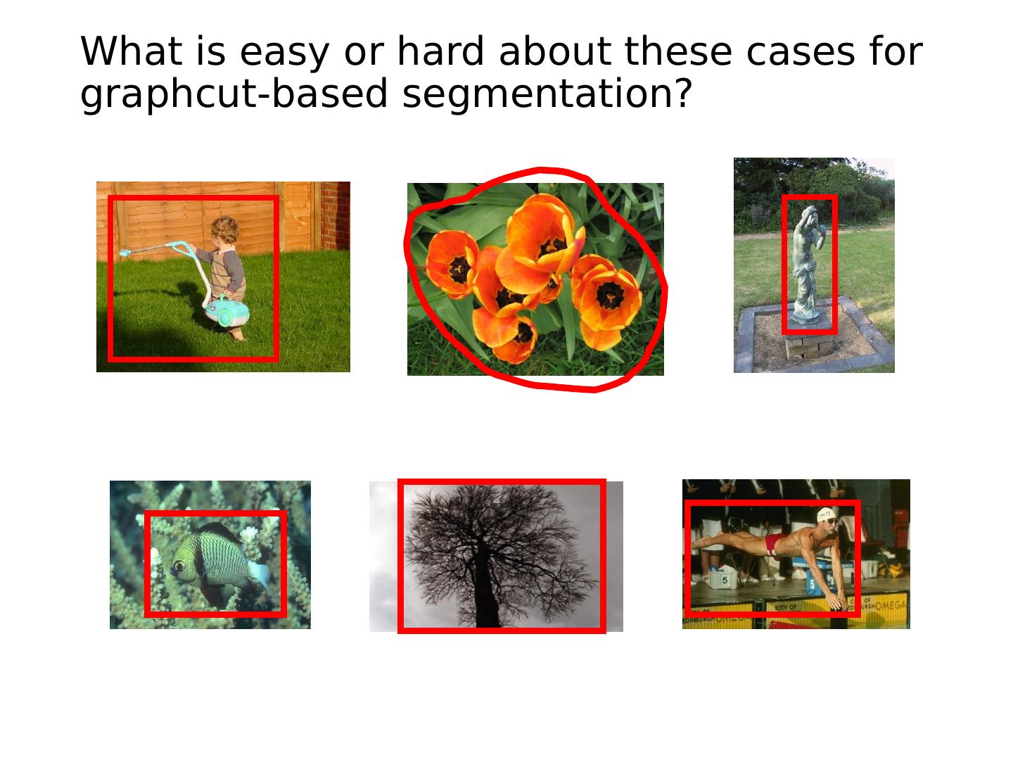
24 .What is easy or hard about these cases for graphcut -based segmentation?

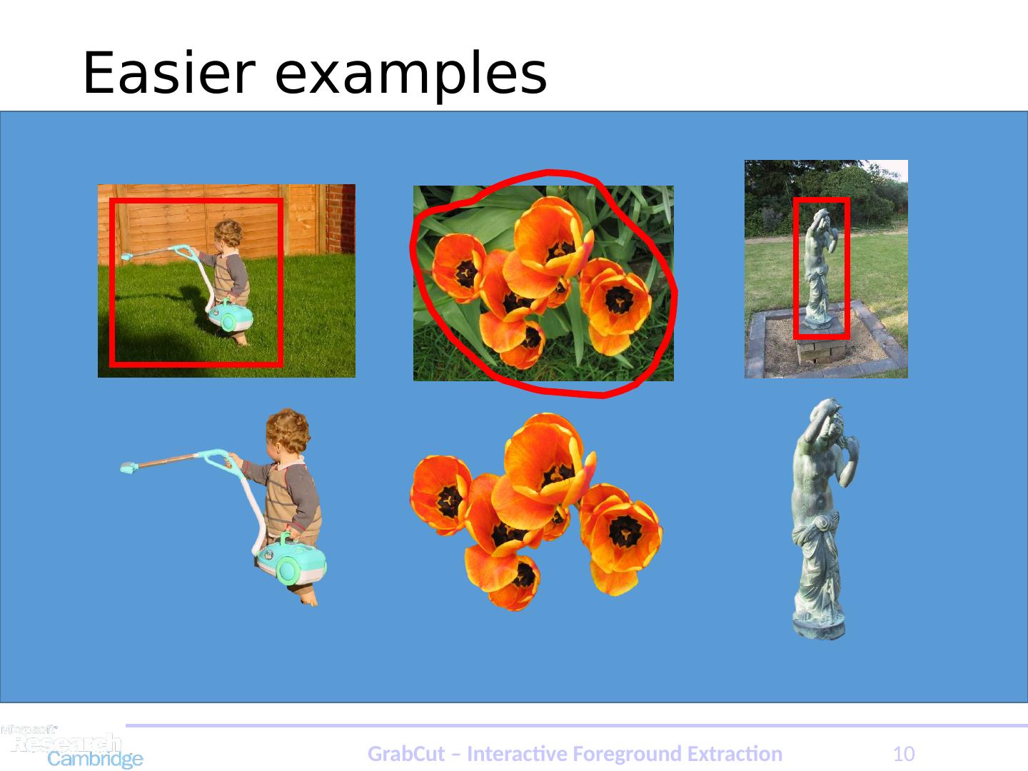
25 .Easier examples GrabCut – Interactive Foreground Extraction 10

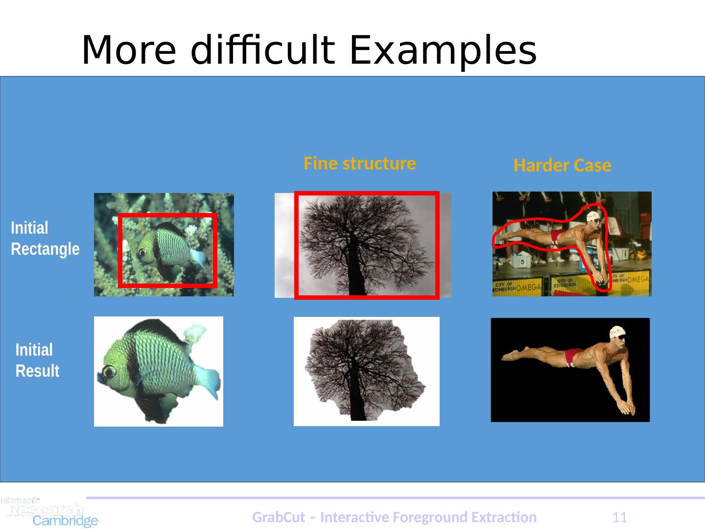
26 . More difficult Examples Camouflage & Low Contrast Harder Case Fine structure Initial Rectangle Initial Result GrabCut – Interactive Foreground Extraction 11

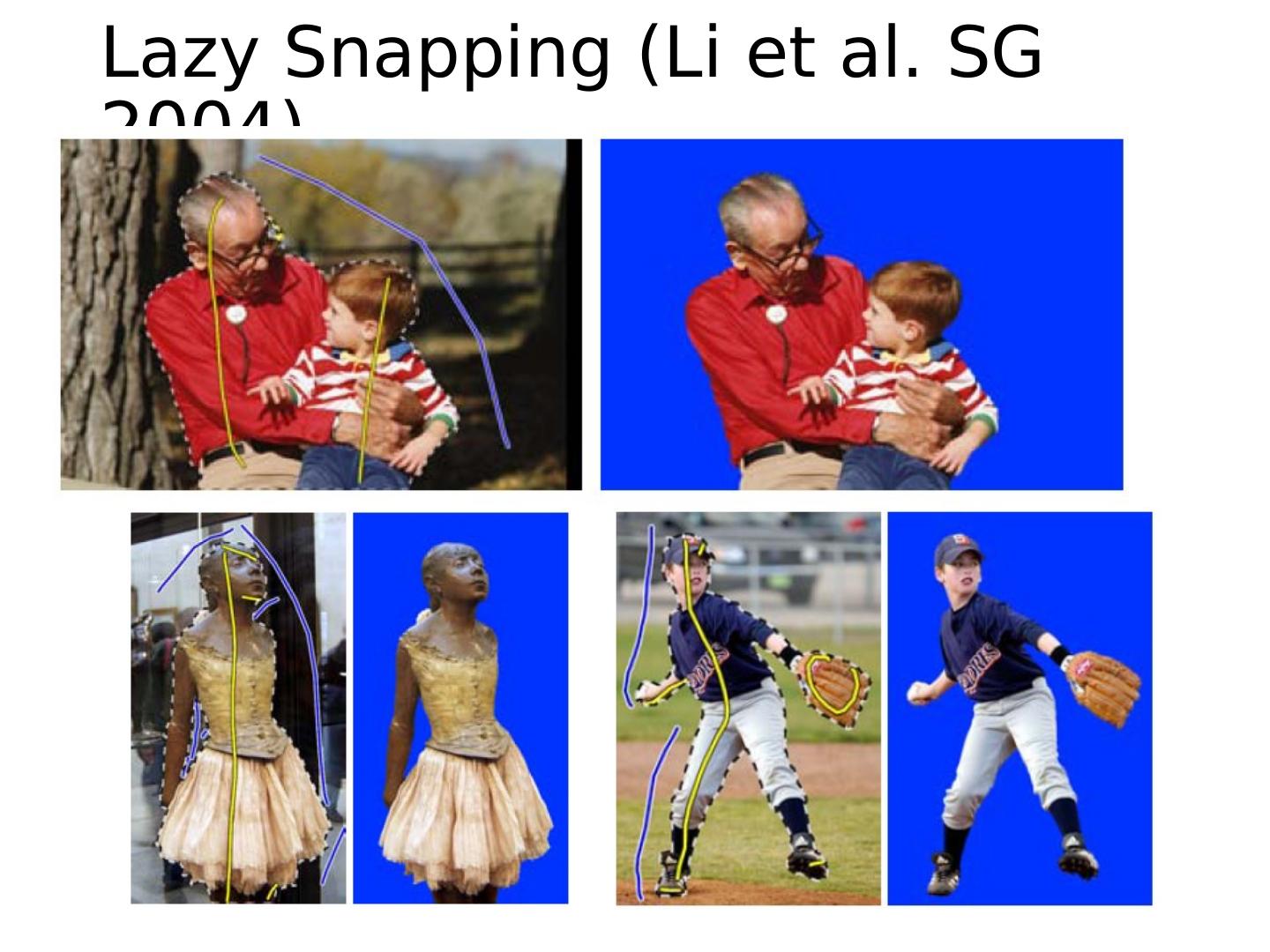
27 .Lazy Snapping (Li et al. SG 2004)

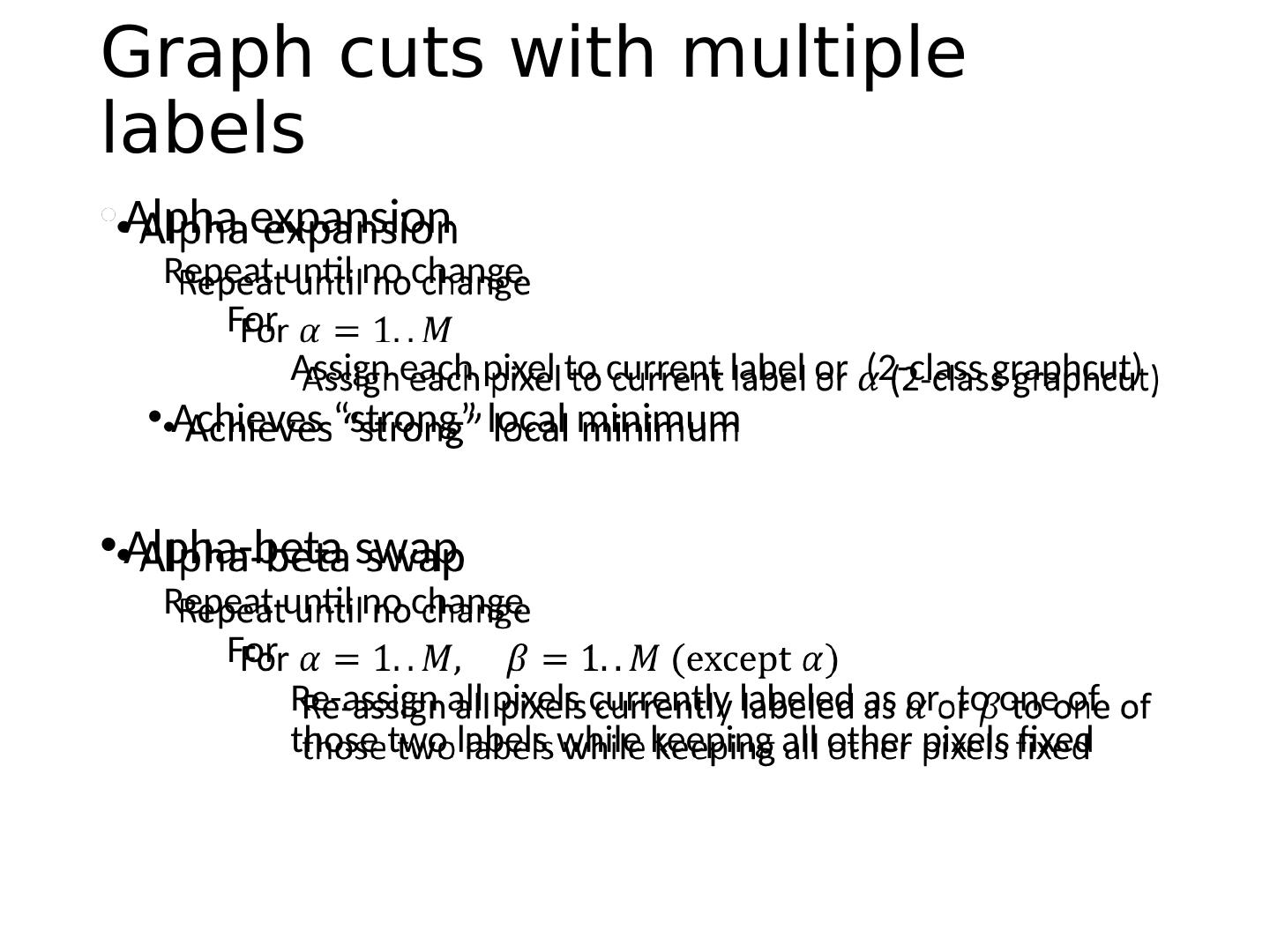
28 .Graph cuts with multiple labels Alpha expansion Repeat until no change F or Assign each pixel to current label or (2-class graphcut ) Achieves “strong” local minimum Alpha-beta swap Repeat until no change For Re-assign all pixels currently labeled as or to one of those two labels while keeping all other pixels fixed  

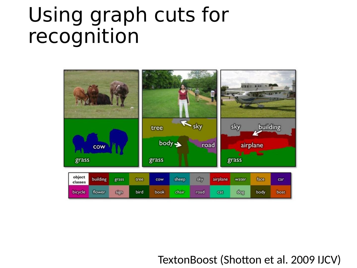
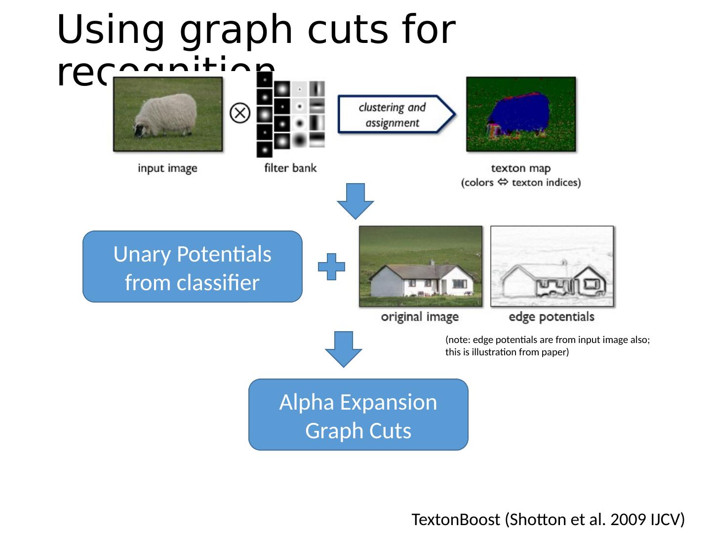
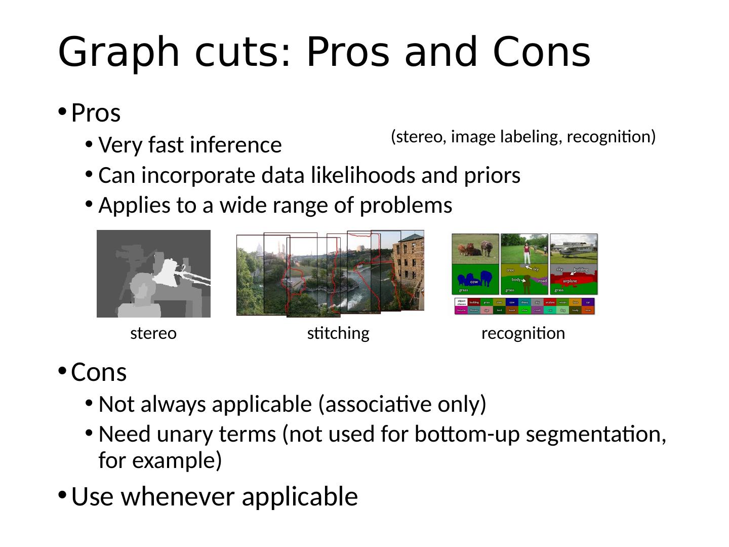
29 .Using graph cuts for recognition TextonBoost ( Shotton et al. 2009 IJCV)