linear,ridge regression, and principal component analysis

1 .Linear, Ridge Regression, and Principal Component Analysis Linear, Ridge Regression, and Principal Component Analysis Jia Li Department of Statistics The Pennsylvania State University Email: jiali@stat.psu.edu http://www.stat.psu.edu/∼jiali Jia Li http://www.stat.psu.edu/∼jiali 

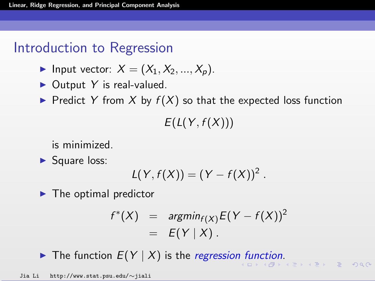
2 .Linear, Ridge Regression, and Principal Component Analysis Introduction to Regression Input vector: X = (X1 , X2 , ..., Xp ). Output Y is real-valued. Predict Y from X by f (X ) so that the expected loss function E (L(Y , f (X ))) is minimized. Square loss: L(Y , f (X )) = (Y − f (X ))2 . The optimal predictor f ∗ (X ) = argminf (X ) E (Y − f (X ))2 = E (Y | X ) . The function E (Y | X ) is the regression function. Jia Li http://www.stat.psu.edu/∼jiali 

3 .Linear, Ridge Regression, and Principal Component Analysis Example The number of active physicians in a Standard Metropolitan Statistical Area (SMSA), denoted by Y , is expected to be related to total population (X1 , measured in thousands), land area (X2 , measured in square miles), and total personal income (X3 , measured in millions of dollars). Data are collected for 141 SMSAs, as shown in the following table. i: 1 2 3 ... 139 140 141 X1 9387 7031 7017 ... 233 232 231 X2 1348 4069 3719 ... 1011 813 654 X3 72100 52737 54542 ... 1337 1589 1148 Y 25627 15389 13326 ... 264 371 140 Goal: Predict Y from X1 , X2 , and X3 . Jia Li http://www.stat.psu.edu/∼jiali 

4 .Linear, Ridge Regression, and Principal Component Analysis Linear Methods The linear regression model p f (X ) = β0 + Xj βj . j=1 What if the model is not true? It is a good approximation Because of the lack of training data/or smarter algorithms, it is the most we can extract robustly from the data. Comments on Xj : Quantitative inputs Transformations of quantitative inputs, e.g., log(·), (·). Basis expansions: X2 = X12 , X3 = X13 , X3 = X1 · X2 . Jia Li http://www.stat.psu.edu/∼jiali 

5 .Linear, Ridge Regression, and Principal Component Analysis Jia Li http://www.stat.psu.edu/∼jiali 

6 .Linear, Ridge Regression, and Principal Component Analysis Estimation The issue of finding the regression function E (Y | X ) is converted to estimating βj , j = 0, 1, ..., p. Training data: {(x1 , y1 ), (x2 , y2 ), ..., (xN , yN )}, where xi = (xi1 , xi2 , ..., xip ) . Denote β = (β0 , β1 , ..., βp )T . The loss function E (Y − f (X ))2 is approximated by the empirical loss RSS(β)/N: N N p RSS(β) = (yi − f (xi ))2 = (yi − β0 − xij βj )2 . i=1 i=1 j=1 Jia Li http://www.stat.psu.edu/∼jiali 

7 .Linear, Ridge Regression, and Principal Component Analysis Notation The input matrix X of dimension N × (p + 1):   1 x1,1 x1,2 ... x1,p  1 x2,1 x2,2 ... x2,p     ... ... ... ... ...  1 xN,1 xN,2 ... xN,p Output vector y:  y1  y2  y=   ...  yN Jia Li http://www.stat.psu.edu/∼jiali 

8 .Linear, Ridge Regression, and Principal Component Analysis ˆ The estimated β is β. The fitted values at the training inputs: p yˆi = βˆ0 + xij βˆj j=1 and   yˆ1  yˆ2  yˆ =    ...  yˆN Jia Li http://www.stat.psu.edu/∼jiali 

9 .Linear, Ridge Regression, and Principal Component Analysis Point Estimate The least square estimation of βˆ is ✞ ☎ βˆ = (XT X)−1 XT y ✝ ✆ The fitted value vector is ✞ ☎ yˆ = Xβˆ = X(XT X)−1 XT y ✝ ✆ Hat matrix: ✞ ☎ H= X(XT X)−1 XT ✝ ✆ Jia Li http://www.stat.psu.edu/∼jiali 

10 .Linear, Ridge Regression, and Principal Component Analysis Geometric Interpretation Each column of X is a vector in an N-dimensional space (NOT the p-dimensional feature vector space). X = (x0 , x1 , ..., xp ) The fitted output vector yˆ is a linear combination of the column vectors xj , j = 0, 1, ..., p. yˆ lies in the subspace spanned by xj , j = 0, 1, ..., p. RSS(β) ˆ = y − yˆ 2 . y − yˆ is perpendicular to the subspace, i.e., yˆ is the projection of y on the subspace. The geometric interpretation is very helpful for understanding coefficient shrinkage and subset selection. Jia Li http://www.stat.psu.edu/∼jiali 

11 .Linear, Ridge Regression, and Principal Component Analysis Jia Li http://www.stat.psu.edu/∼jiali 

12 .Linear, Ridge Regression, and Principal Component Analysis Example Results for the SMSA Problem Yˆi = −143.89 + 0.341Xi1 − 0.0193Xi2 + 0.255Xi3 . RSS(β)ˆ = 52942336. Jia Li http://www.stat.psu.edu/∼jiali 

13 .Linear, Ridge Regression, and Principal Component Analysis If the Linear Model Is True E (Y | X ) = β0 + pj=1 Xj βj The least square estimation of β is unbiased, E (βˆj ) = βj j = 0, 1, ..., p . To draw inferences about β, further assume: Y = E (Y | X ) + where ∼ N(0, σ 2 ) and is independent of X . Xij are regarded as fixed, Yi are random due to . Estimation accuracy: Var (β)ˆ = (XT X)−1 σ 2 . Under the assumption, βˆ ∼ N(β, (XT X)−1 σ 2 ) . Confidence intervals can be computed and significant tests can be done. Jia Li http://www.stat.psu.edu/∼jiali 

14 .Linear, Ridge Regression, and Principal Component Analysis Gauss-Markov Theorem Assume the linear model is true. For any linear combination of the parameters β0 ,...,βp , denoted by θ = aT β, aT βˆ is an unbiased estimation since βˆ is unbiased. The least squares estimate of θ is θˆ = aT βˆ = aT (XT X)−1 Xy ˜aT y , which is linear in y. Jia Li http://www.stat.psu.edu/∼jiali 

15 .Linear, Ridge Regression, and Principal Component Analysis Suppose c T y is another unbiased linear estimate of θ, i.e., E (c T y) = θ. The least square estimate yields the minimum variance among all linear unbiased estimate. Var (˜aT y) ≤ Var (c T y) . βj , j = 0, 1, ..., p are special cases of aT β, where aT only has one non-zero element that equals 1. Jia Li http://www.stat.psu.edu/∼jiali 

16 .Linear, Ridge Regression, and Principal Component Analysis Subset Selection and Coefficient Shrinkage Biased estimation may yield better prediction accuracy. ˆ For β˜ = βˆ , a ≥ 1, Squared loss: E (βˆ − 1)2 = Var (β). a E (β˜ − 1)2 = Var (β) ˜ + (E (β) ˜ − 1)2 = 12 + ( 1 − 1)2 . a a Practical consideration: interpretation. Sometimes, we are not satisfied with a “black box”. Jia Li http://www.stat.psu.edu/∼jiali 

17 .Linear, Ridge Regression, and Principal Component Analysis Assume βˆ ∼ N(1, 1). The squared error loss is reduced by shrinking the estimation. Jia Li http://www.stat.psu.edu/∼jiali 

18 .Linear, Ridge Regression, and Principal Component Analysis Subset Selection To choose k predicting variables from the total of p variables, ˆ search for the subset yielding minimum RSS(β). Forward stepwise selection: start with the intercept, then sequentially adds into the model the predictor that most improves the fit. Backward stepwise selection: start with the full model, and sequentially deletes predictors. How to choose k: stop forward or backward stepwise selection when no predictor produces the F -ratio statistic greater than a threshold. Jia Li http://www.stat.psu.edu/∼jiali 

19 .Linear, Ridge Regression, and Principal Component Analysis Ridge Regression Centered inputs Suppose xj , j = 1, ..., p, are mean removed. βˆ0 = y¯ = N yi /N. i=1 If we remove the mean of yi , we can assume p E (Y | X ) = βj Xj j=1 Input matrix X has p (rather than p + 1) columns. βˆ = (XT X)−1 XT y yˆ = X(XT X)−1 XT y Jia Li http://www.stat.psu.edu/∼jiali 

20 .Linear, Ridge Regression, and Principal Component Analysis Singular Value Decomposition (SVD) If the column vectors of X are orthonormal, i.e., the variables Xj , j = 1, 2, ..., p, are uncorrelated and have unit norm. βˆj are the coordinates of y on the orthonormal basis X. In general ✞ ☎ T ✝X = UDV ✆. U = (u1 , u2 , ..., up ) is an N × p orthogonal matrix. uj , j = 1, ..., p form an orthonormal basis for the space spanned by the column vectors of X. V = (v1 , v2 , ..., vp ) is an p × p orthogonal matrix. vj , j = 1, ..., p form an orthonormal basis for the space spanned by the row vectors of X. D = diag (d1 , d2 , ..., dp ), d1 ≥ d2 ≥ ... ≥ dp ≥ 0 are the singular values of X. Jia Li http://www.stat.psu.edu/∼jiali 

21 .Linear, Ridge Regression, and Principal Component Analysis Principal Components The sample covariance matrix of X is S = XT X/N . Eigen decomposition of XT X: XT X = (UDVT )T (UDVT ) = VDUT UDVT = VD2 VT The eigenvectors of XT X, vj , are called principal component direction of X. Jia Li http://www.stat.psu.edu/∼jiali 

22 .Linear, Ridge Regression, and Principal Component Analysis It’s easy to see that zj = Xvj = uj dj . Hence uj , is simply the projection of the row vectors of X, i.e., the input predictor vectors, on the direction vj , scaled by dj . For example   X1,1 v1,1 + X1,2 v1,2 + · · · + X1,p v1,p  X2,1 v1,1 + X2,2 v1,2 + · · · + X2,p v1,p  z1 =    .. .. ..   . . .  XN,1 v1,1 + XN,2 v1,2 + · · · + XN,p v1,p The principal components of X are zj = dj uj , j = 1, ..., p. The first principal component of X, z1 , has the largest sample variance amongst all normalized linear combinations of the columns of X. Var (z1 ) = d12 /N . Subsequent principal components zj have maximum variance dj2 /N, subject to being orthogonal to the earlier ones. Jia Li http://www.stat.psu.edu/∼jiali 

23 .Linear, Ridge Regression, and Principal Component Analysis Jia Li http://www.stat.psu.edu/∼jiali 

24 .Linear, Ridge Regression, and Principal Component Analysis Ridge Regression Minimize a penalized residual sum of squares    N p p  βˆridge = argminβ (yi − β0 − xij βj )2 + λ βj2   i=1 j=1 j=1 Equivalently N p βˆridge = argminβ (yi − β0 − xij βj )2 i=1 j=1 p subject to βj2 ≤ s . j=1 λ or s controls the model complexity. Jia Li http://www.stat.psu.edu/∼jiali 

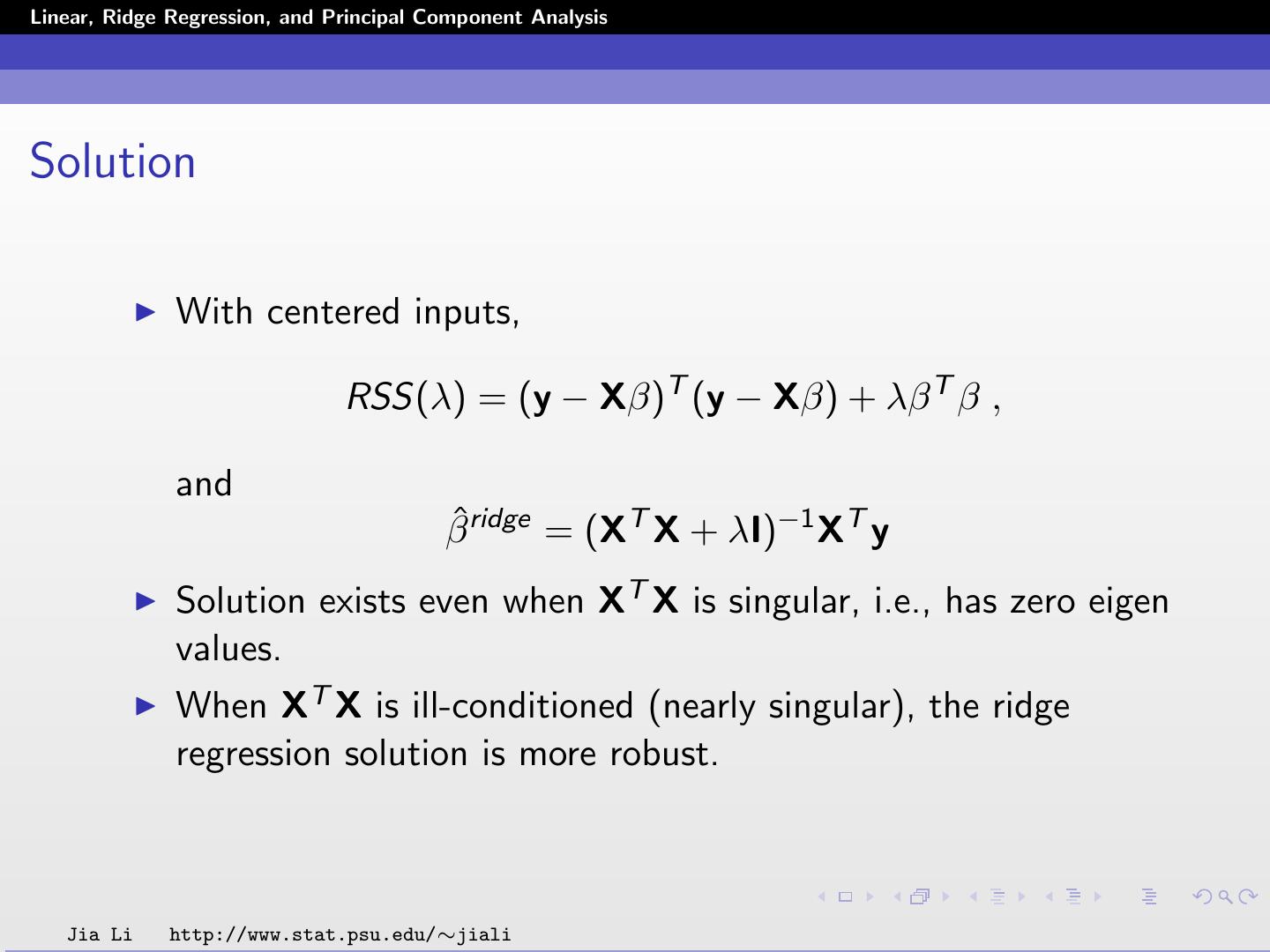
25 .Linear, Ridge Regression, and Principal Component Analysis Solution With centered inputs, RSS(λ) = (y − Xβ)T (y − Xβ) + λβ T β , and βˆridge = (XT X + λI)−1 XT y Solution exists even when XT X is singular, i.e., has zero eigen values. When XT X is ill-conditioned (nearly singular), the ridge regression solution is more robust. Jia Li http://www.stat.psu.edu/∼jiali 

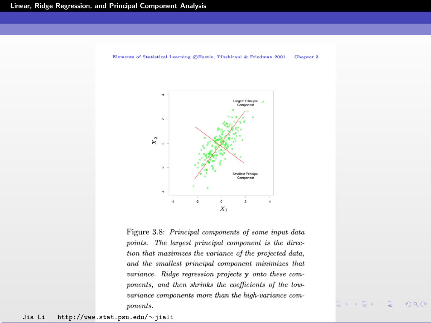
26 .Linear, Ridge Regression, and Principal Component Analysis Geometric Interpretation Center inputs. Consider the fitted response yˆ = Xβˆridge = X(XT X + λI)−1 XT y = UD(D2 + λI)−1 DUT y p dj2 = uj uT j y , dj2 + λ j=1 where uj are the normalized principal components of X. Ridge regression shrinks the coordinates with respect to the orthonormal basis formed by the principal components. Coordinate with respect to the principal component with a smaller variance is shrunk more. Jia Li http://www.stat.psu.edu/∼jiali 

27 .Linear, Ridge Regression, and Principal Component Analysis Instead of using X = (X1 , X2 , ..., Xp ) as predicting variables, use the transformed variables (X v1 , X v2 , ..., X vp ) as predictors. ˜ = UD (Note X = UDVT ). The input matrix is X Then for the new inputs dj σ2 βˆjridge = uT y , Var (βˆj ) = 2 dj + λ j 2 dj where σ 2 is the variance of the error term in the linear model. The factor of shrinkage given by ridge regression is dj2 . dj2 + λ Jia Li http://www.stat.psu.edu/∼jiali 

28 .Linear, Ridge Regression, and Principal Component Analysis The Geometric interpretation of principal components and shrinkage by ridge regression. Jia Li http://www.stat.psu.edu/∼jiali 

29 .Linear, Ridge Regression, and Principal Component Analysis Compare squared loss E (βj − βˆj )2 Without shrinkage: σ 2 /dj2 . With shrinkage: Bias 2 + Variance. dj2 σ2 dj2 2 (βj − βj · )2 + · ( ) dj2 + λ dj2 dj2 + λ 2 2 2 j β2 σ 2 dj (dj + λ σ2 ) = · dj2 (dj2 + λ)2 Consider the ratio between squared loss β2 dj2 (dj2 + λ2 σj2 ) . (dj2 + λ)2 Jia Li http://www.stat.psu.edu/∼jiali