Apache Spark2.3中直方图的基数估计

1 .Cardinality Estimation through Histogram in Apache Spark 2.3 Ron Hu, Zhenhua Wang Huawei Technologies, Inc. #DevSAIS13 

2 .Agenda • Catalyst Architecture • Cost Based Optimizer in Spark 2.2 • Statistics Collected • Histogram Support in Spark 2.3 • Configuration Parameters • Q&A 2 

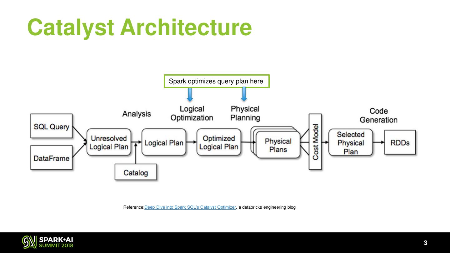
3 .Catalyst Architecture Spark optimizes query plan here Reference:Deep Dive into Spark SQL’s Catalyst Optimizer, a databricks engineering blog 3 

4 .Query Optimizer in Spark SQL • Spark SQL’s query optimizer is based on both rules and cost. • Most of Spark SQL optimizer’s rules are heuristics rules. – PushDownPredicate, ColumnPruning, ConstantFolding,…. • Cost based optimization (CBO) was added in Spark 2.2. 4 

5 .Cost Based Optimizer in Spark 2.2 • It was a good and working CBO framework to start with. • Focused on – Statistics collection, – Cardinality estimation, – Build side selection, broadcast vs. shuffled join, join reordering, etc. • Used heuristics formula for cost function in terms of cardinality and data size of each operator. 5 

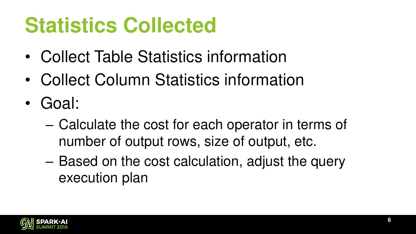
6 .Statistics Collected • Collect Table Statistics information • Collect Column Statistics information • Goal: – Calculate the cost for each operator in terms of number of output rows, size of output, etc. – Based on the cost calculation, adjust the query execution plan 6 

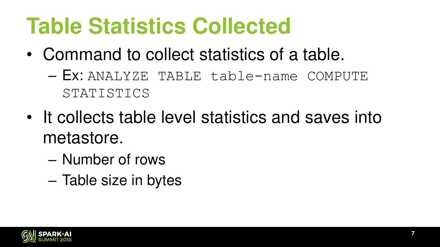
7 .Table Statistics Collected • Command to collect statistics of a table. – Ex: ANALYZE TABLE table-name COMPUTE STATISTICS • It collects table level statistics and saves into metastore. – Number of rows – Table size in bytes 7 

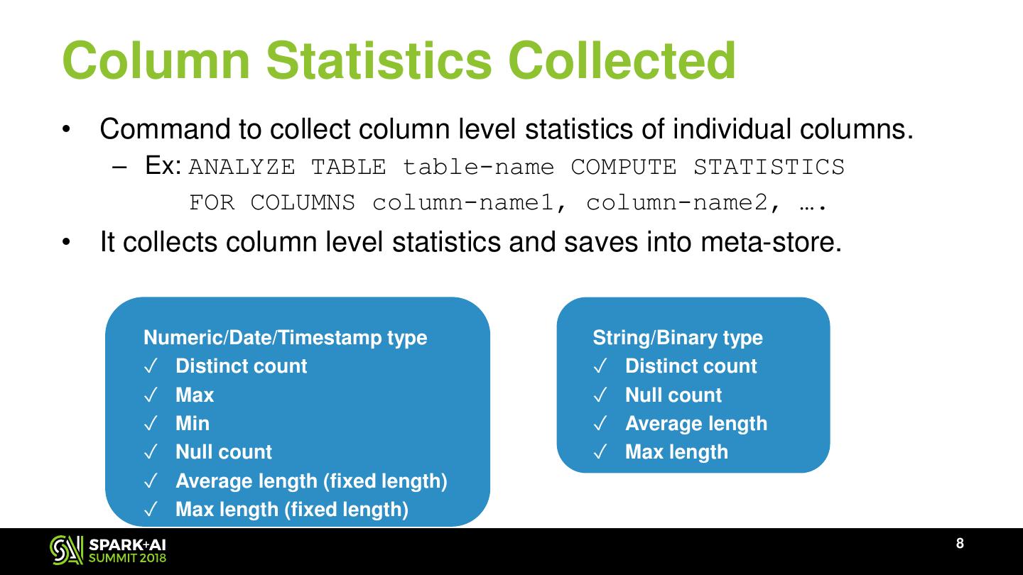
8 .Column Statistics Collected • Command to collect column level statistics of individual columns. – Ex: ANALYZE TABLE table-name COMPUTE STATISTICS FOR COLUMNS column-name1, column-name2, …. • It collects column level statistics and saves into meta-store. Numeric/Date/Timestamp type String/Binary type ✓ Distinct count ✓ Distinct count ✓ Max ✓ Null count ✓ Min ✓ Average length ✓ Null count ✓ Max length ✓ Average length (fixed length) ✓ Max length (fixed length) 8 

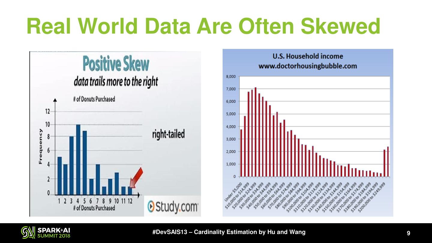
9 .Real World Data Are Often Skewed #DevSAIS13 – Cardinality Estimation by Hu and Wang 9 

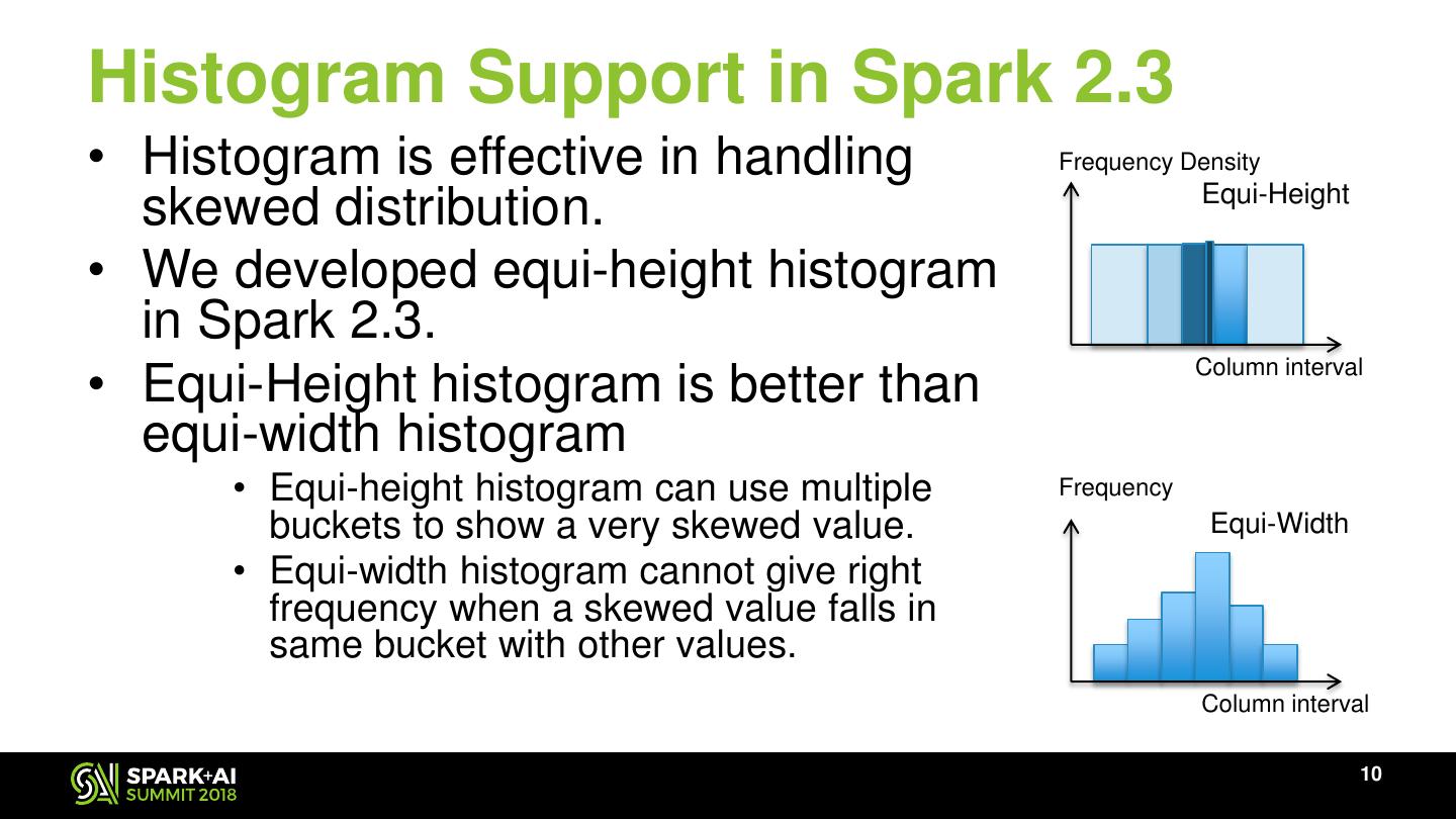
10 .Histogram Support in Spark 2.3 • Histogram is effective in handling Frequency Density Equi-Height skewed distribution. • We developed equi-height histogram in Spark 2.3. • Equi-Height histogram is better than Column interval equi-width histogram • Equi-height histogram can use multiple Frequency buckets to show a very skewed value. Equi-Width • Equi-width histogram cannot give right frequency when a skewed value falls in same bucket with other values. Column interval 10 

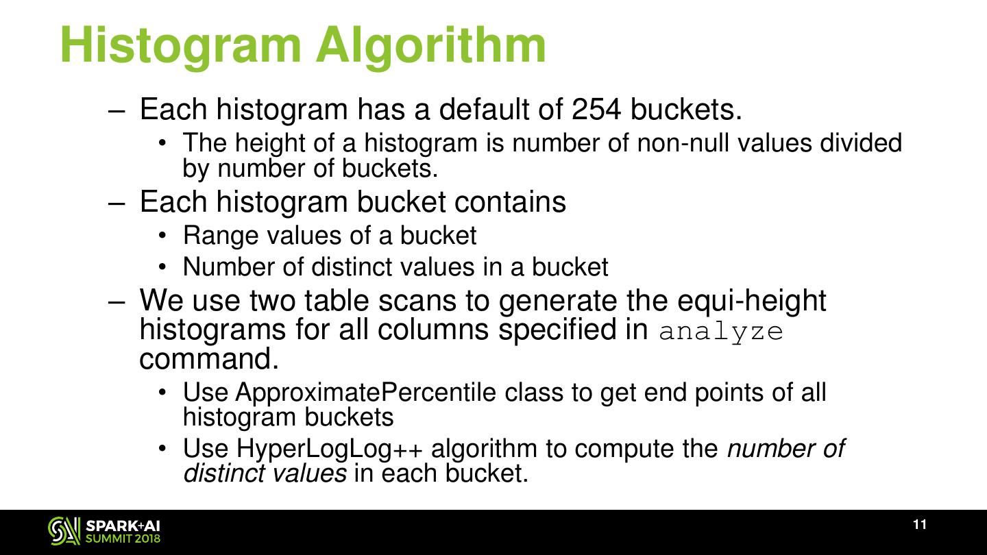
11 .Histogram Algorithm – Each histogram has a default of 254 buckets. • The height of a histogram is number of non-null values divided by number of buckets. – Each histogram bucket contains • Range values of a bucket • Number of distinct values in a bucket – We use two table scans to generate the equi-height histograms for all columns specified in analyze command. • Use ApproximatePercentile class to get end points of all histogram buckets • Use HyperLogLog++ algorithm to compute the number of distinct values in each bucket. 11 

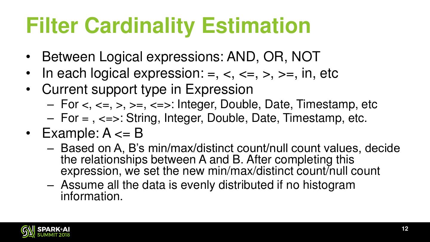
12 .Filter Cardinality Estimation • Between Logical expressions: AND, OR, NOT • In each logical expression: =, <, <=, >, >=, in, etc • Current support type in Expression – For <, <=, >, >=, <=>: Integer, Double, Date, Timestamp, etc – For = , <=>: String, Integer, Double, Date, Timestamp, etc. • Example: A <= B – Based on A, B’s min/max/distinct count/null count values, decide the relationships between A and B. After completing this expression, we set the new min/max/distinct count/null count – Assume all the data is evenly distributed if no histogram information. 12 

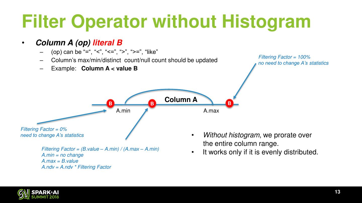
13 .Filter Operator without Histogram • Column A (op) literal B – (op) can be “=“, “<”, “<=”, “>”, “>=”, “like” Filtering Factor = 100% – Column’s max/min/distinct count/null count should be updated no need to change A’s statistics – Example: Column A < value B B Column A B A.min A.max Filtering Factor = 0% need to change A’s statistics • Without histogram, we prorate over the entire column range. Filtering Factor = (B.value – A.min) / (A.max – A.min) A.min = no change • It works only if it is evenly distributed. A.max = B.value A.ndv = A.ndv * Filtering Factor 13 

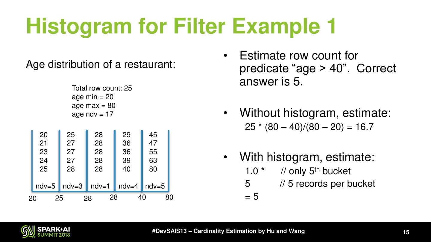
14 .Filter Operator with Histogram • With histogram, we check the range values of a bucket to see if it should be included in estimation. • We prorate only the boundary bucket. • This way can enhance the accuracy of estimation since we prorate (or guess) only a much smaller set of records in a bucket only. 14 

15 .Histogram for Filter Example 1 • Estimate row count for Age distribution of a restaurant: predicate “age > 40”. Correct Total row count: 25 answer is 5. age min = 20 age max = 80 age ndv = 17 • Without histogram, estimate: 25 * (80 – 40)/(80 – 20) = 16.7 20 25 28 29 45 21 27 28 36 47 23 27 28 36 55 24 27 28 39 63 • With histogram, estimate: 25 28 28 40 80 1.0 * // only 5th bucket ndv=5 ndv=3 ndv=1 ndv=4 ndv=5 5 // 5 records per bucket 20 25 28 28 40 80 =5 #DevSAIS13 – Cardinality Estimation by Hu and Wang 15 

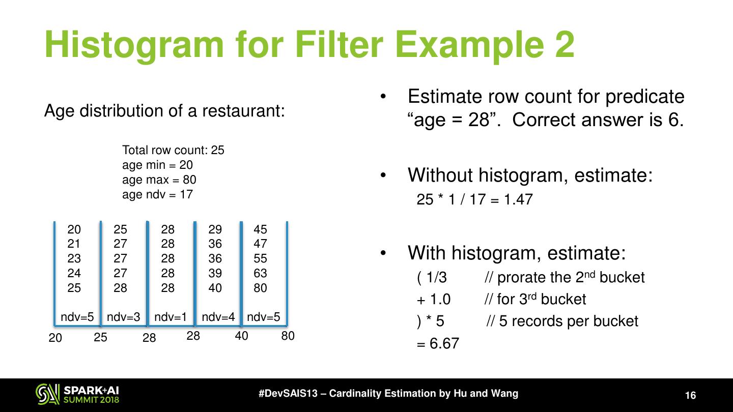
16 .Histogram for Filter Example 2 • Estimate row count for predicate Age distribution of a restaurant: “age = 28”. Correct answer is 6. Total row count: 25 age min = 20 age max = 80 • Without histogram, estimate: age ndv = 17 25 * 1 / 17 = 1.47 20 25 28 29 45 21 27 28 36 47 23 27 28 36 55 • With histogram, estimate: 24 27 28 39 63 ( 1/3 // prorate the 2nd bucket 25 28 28 40 80 + 1.0 // for 3rd bucket ndv=5 ndv=3 ndv=1 ndv=4 ndv=5 )*5 // 5 records per bucket 20 25 28 28 40 80 = 6.67 #DevSAIS13 – Cardinality Estimation by Hu and Wang 16 

17 .Join Cardinality without Histogram • Inner-Join: The number of rows of “A join B on A.k1 = B.k1” is estimated as: num(A ⟗ B) = num(A) * num(B) / max(distinct(A.k1), distinct(B.k1)), – where num(A) is the number of records in table A, distinct is the number of distinct values of that column. – The underlying assumption for this formula is that each value of the smaller domain is included in the larger domain. – Assuming uniform distribution for entire range of both join columns. • We similarly estimate cardinalities for Left-Outer Join, Right-Outer Join and Full-Outer Join 17 

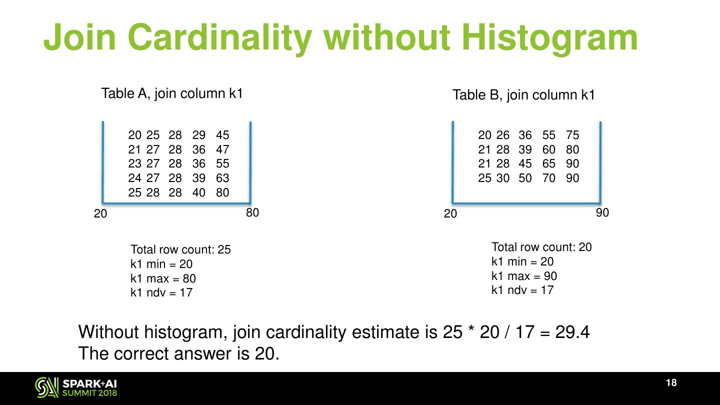
18 .Join Cardinality without Histogram Table A, join column k1 Table B, join column k1 20 25 28 29 45 20 26 36 55 75 21 27 28 36 47 21 28 39 60 80 23 27 28 36 55 21 28 45 65 90 24 27 28 39 63 25 30 50 70 90 25 28 28 40 80 20 80 20 90 Total row count: 25 Total row count: 20 k1 min = 20 k1 min = 20 k1 max = 80 k1 max = 90 k1 ndv = 17 k1 ndv = 17 Without histogram, join cardinality estimate is 25 * 20 / 17 = 29.4 The correct answer is 20. 18 

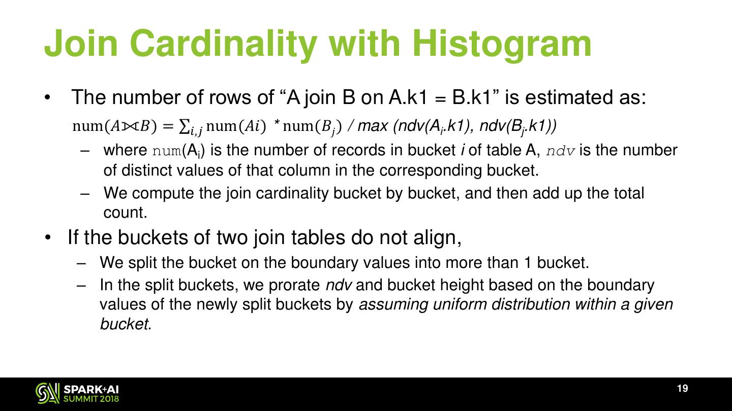
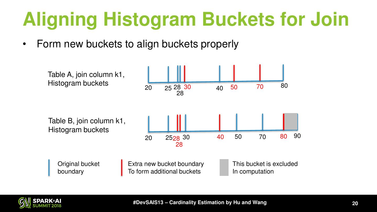
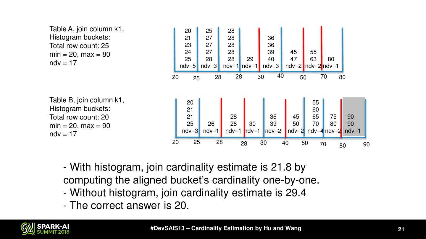
19 .Join Cardinality with Histogram • The number of rows of “A join B on A.k1 = B.k1” is estimated as: num(𝐴⟗𝐵) = 𝑖,𝑗 num(𝐴𝑖) * num(𝐵𝑗) / max (ndv(Ai.k1), ndv(Bj.k1)) – where num(Ai) is the number of records in bucket i of table A, ndv is the number of distinct values of that column in the corresponding bucket. – We compute the join cardinality bucket by bucket, and then add up the total count. • If the buckets of two join tables do not align, – We split the bucket on the boundary values into more than 1 bucket. – In the split buckets, we prorate ndv and bucket height based on the boundary values of the newly split buckets by assuming uniform distribution within a given bucket. 19 

20 .Aligning Histogram Buckets for Join • Form new buckets to align buckets properly Table A, join column k1, Histogram buckets 70 80 20 25 28 30 40 50 28 Table B, join column k1, Histogram buckets 20 25 28 30 40 50 70 80 90 28 Original bucket Extra new bucket boundary This bucket is excluded boundary To form additional buckets In computation #DevSAIS13 – Cardinality Estimation by Hu and Wang 20 

21 .Table A, join column k1, 20 25 28 Histogram buckets: 21 27 28 36 Total row count: 25 23 27 28 36 min = 20, max = 80 24 27 28 39 45 55 25 28 28 29 40 47 63 80 ndv = 17 ndv=5 ndv=3 ndv=1 ndv=1 ndv=3 ndv=2 ndv=2 ndv=1 20 25 28 28 30 40 50 70 80 Table B, join column k1, 20 55 Histogram buckets: 21 60 Total row count: 20 21 28 36 45 65 75 90 min = 20, max = 90 25 26 28 30 39 50 70 80 90 ndv=3 ndv=1 ndv=1 ndv=1 ndv=2 ndv=2 ndv=4 ndv=2 ndv=1 ndv = 17 20 25 28 28 30 40 50 70 90 80 - With histogram, join cardinality estimate is 21.8 by computing the aligned bucket’s cardinality one-by-one. - Without histogram, join cardinality estimate is 29.4 - The correct answer is 20. #DevSAIS13 – Cardinality Estimation by Hu and Wang 21 

22 .Other Operator Estimation • Project: does not change row count • Aggregate: consider uniqueness of group-by columns • Limit, Sample, etc. 22 

23 .Statistics Propagation a: newMin, newMax, newNdv … b: newMin, newMax, newNdv … … Top-down statistics Join Bottom-up statistics requests (t1.a = t2.b) propagation b: min, max, ndv … a: min, max, ndv … Scan t1 Scan t2 … … 23 

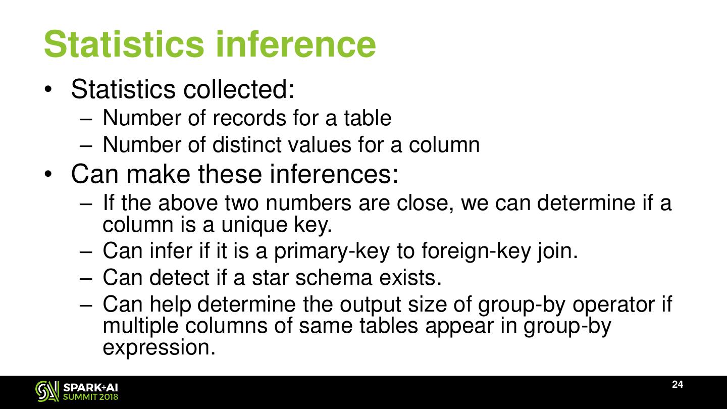
24 .Statistics inference • Statistics collected: – Number of records for a table – Number of distinct values for a column • Can make these inferences: – If the above two numbers are close, we can determine if a column is a unique key. – Can infer if it is a primary-key to foreign-key join. – Can detect if a star schema exists. – Can help determine the output size of group-by operator if multiple columns of same tables appear in group-by expression. 24 

25 .Configuration Parameters Configuration Parameters Default Suggested Value Value spark.sql.cbo.enabled False True spark.sql.cbo.joinReorder.enabled False True spark.sql.cbo.joinReorder.dp.threshold 12 12 spark.sql.cbo.joinReorder.card.weight 0.7 0.7 spark.sql.statistics.size.autoUpdate.enabled False True spark.sql.statistics.histogram.enabled False True spark.sql.statistics.histogram.numBins 254 254 spark.sql.statistics.ndv.maxError 0.05 0.05 spark.sql.statistics.percentile.accuracy 10000 10000 #DevSAIS13 25 

26 .Reference • SPARK-16026: Cost-Based Optimizer Framework – https://issues.apache.org/jira/browse/SPARK-16026 – It has 45 sub-tasks. • SPARK-21975: Histogram support in cost-based optimizer – https://issues.apache.org/jira/browse/SPARK-21975 – It has 10 sub-tasks. #DevSAIS13 – Cardinality Estimation by Hu and Wang 26 

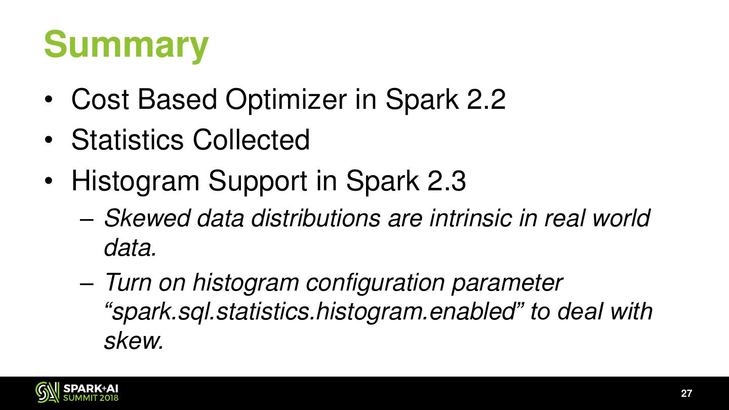
27 .Summary • Cost Based Optimizer in Spark 2.2 • Statistics Collected • Histogram Support in Spark 2.3 – Skewed data distributions are intrinsic in real world data. – Turn on histogram configuration parameter “spark.sql.statistics.histogram.enabled” to deal with skew. 27 

28 .Q&A ron.hu@huawei.com wangzhenhua@huawei.com