数据通信：多路复用和压缩

1 .Chapter 5 Making Connections Efficient: Multiplexing and Compression

2 .Introduction Under the simplest conditions, a medium can carry only one signal at any moment in time For multiple signals to share one medium, the medium must somehow be divided, giving each signal a portion of the total bandwidth. The current techniques that can accomplish this include: Frequency division multiplexing Time division multiplexing Wavelength division multiplexing Discrete Multitone Code division multiplexing

3 .Frequency Division Multiplexing Assignment of non-overlapping frequency ranges to signal on a medium. All signals are transmitted at the same time, each using different frequencies. A multiplexor accepts inputs and assigns frequencies to each device. The multiplexor is attached to a high-speed communications line. A corresponding multiplexor, or demultiplexor, is on the end of the high-speed line and separates the multiplexed signals. Analog signaling is used to transmit signals. Used in broadcast radio and television, cable television, and the AMPS cellular phone systems. More susceptible to noise.

4 .4

5 .Time Division Multiplexing Sharing of the signal is accomplished by dividing available transmission time on a medium among users. Digital signaling. Two basic forms: Synchronous time division multiplexing Statistical time division multiplexing

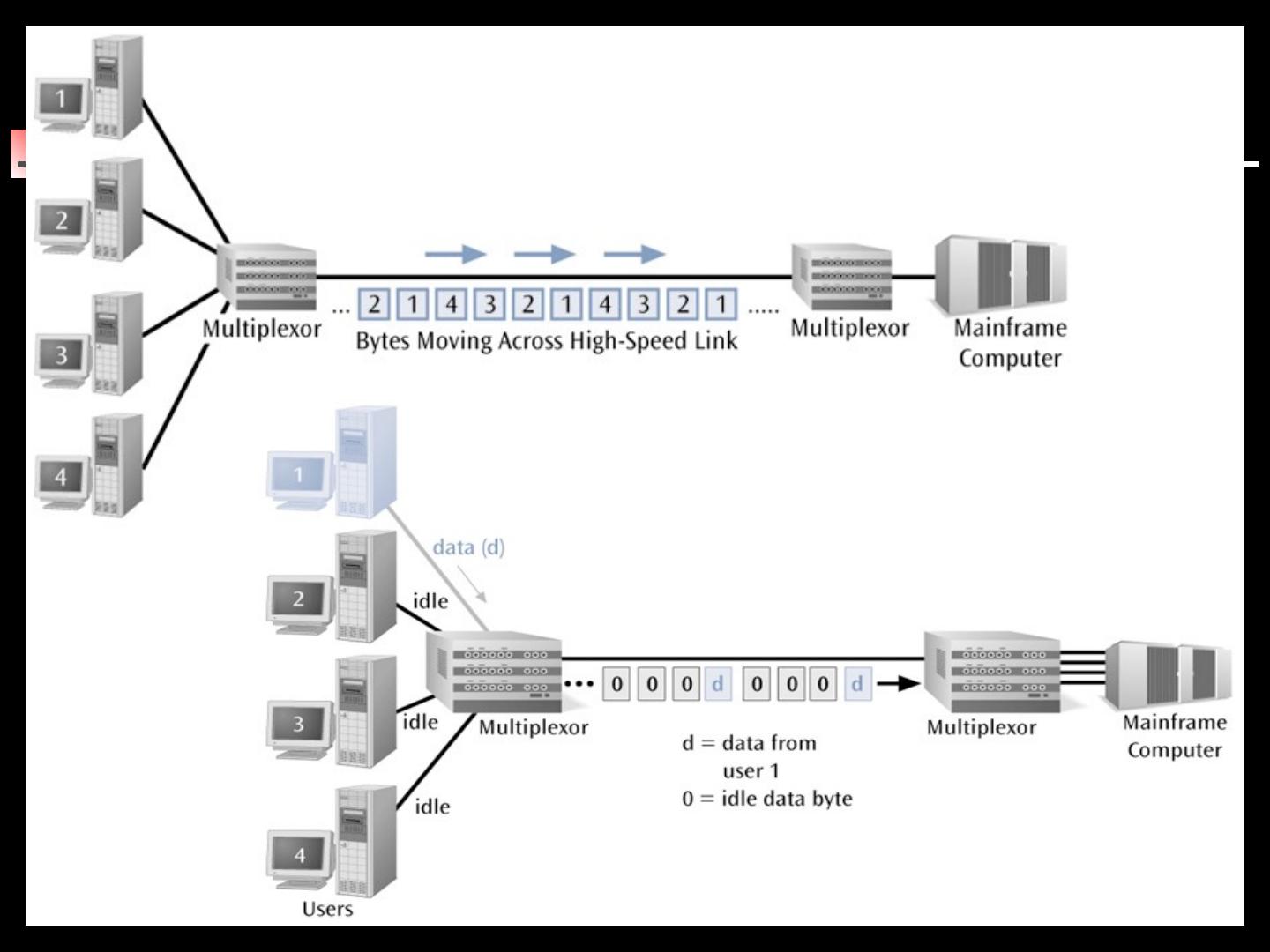
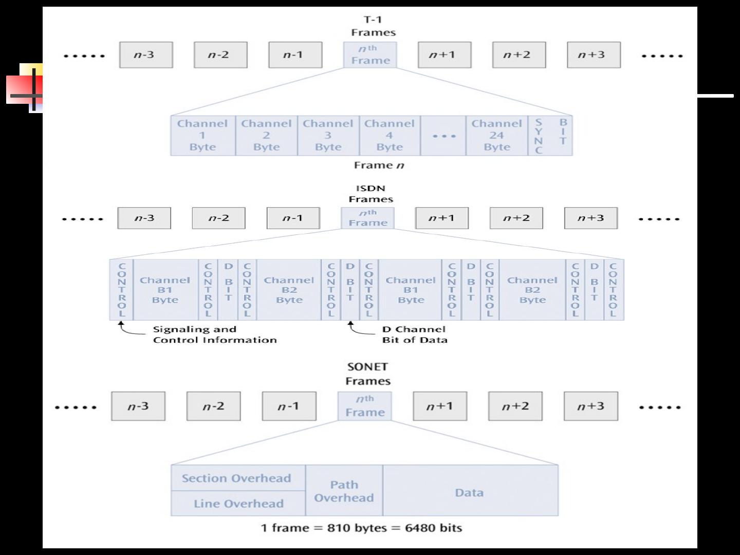
6 .Synchronous Time Division Multiplexing The multiplexor accepts input from attached devices in a round-robin fashion and transmit the data in a never ending pattern. For devices that generate data at a faster rate than other devices, the multiplexor must either: sample the incoming data stream from that device more often than it samples the other devices, or buffer the faster incoming stream. For devices that has nothing to transmit, the multiplexor insert a piece of data from that device into the multiplexed stream. T1, ISDN, and SONET/SDH are common examples of synchronous time division multiplexing.

7 .7

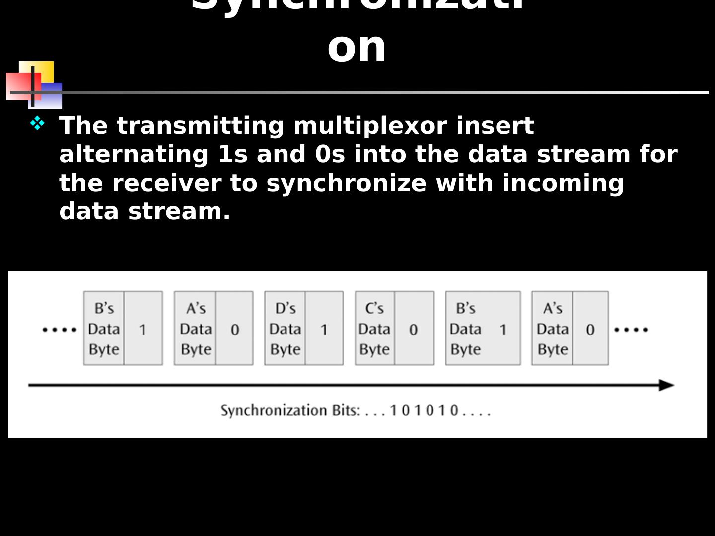
8 .Synchronization The transmitting multiplexor insert alternating 1s and 0s into the data stream for the receiver to synchronize with incoming data stream.

9 .9

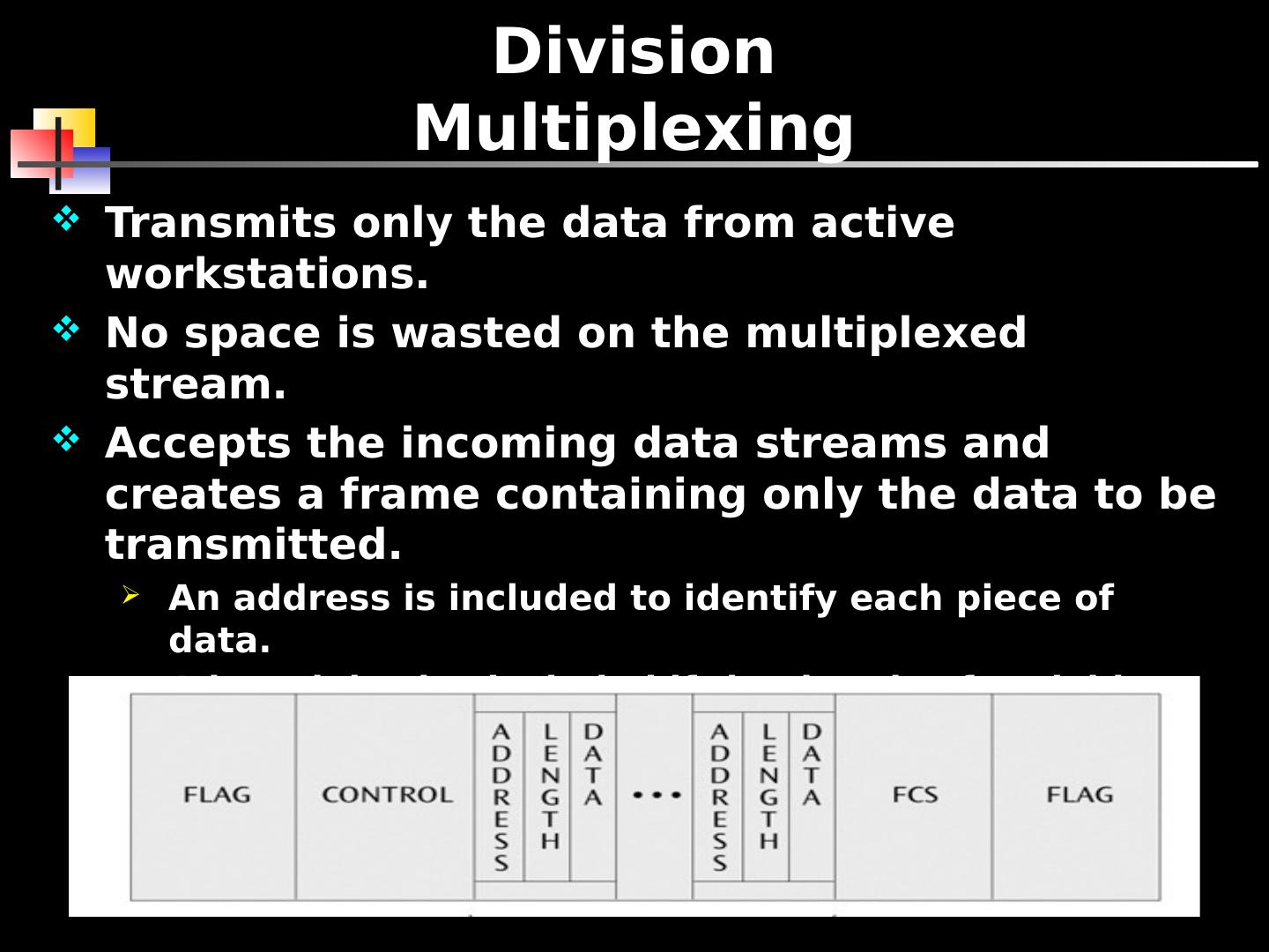
10 .Statistical Time Division Multiplexing Transmits only the data from active workstations. No space is wasted on the multiplexed stream. Accepts the incoming data streams and creates a frame containing only the data to be transmitted. An address is included to identify each piece of data. A length is also included if the data is of variable size. The transmitted frame contains a collection of data groups.

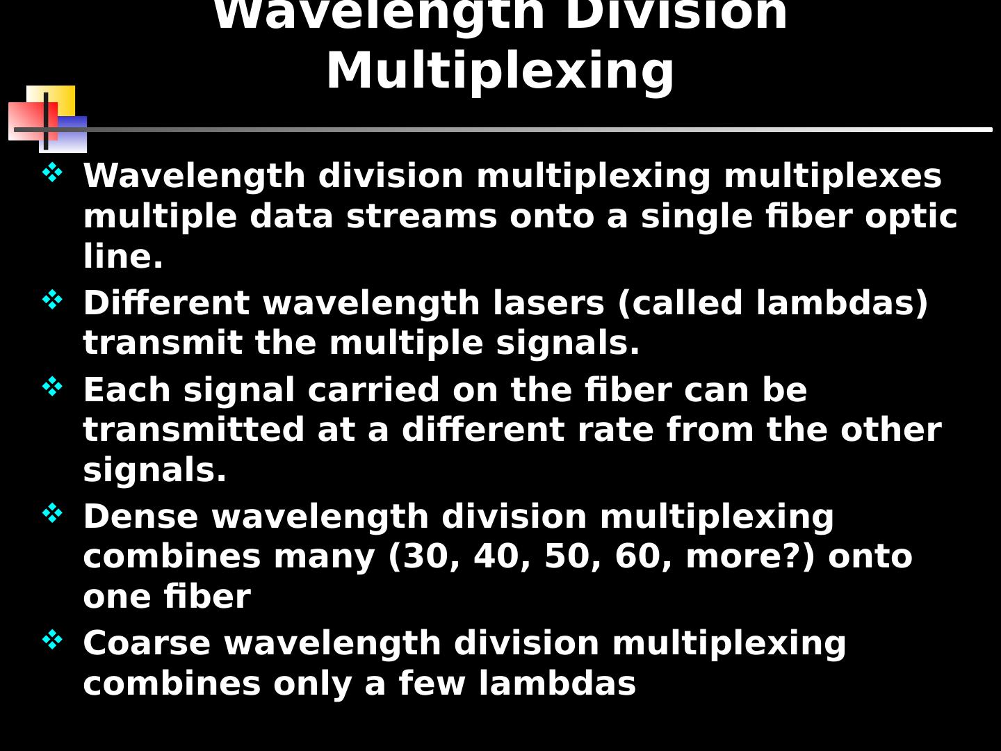
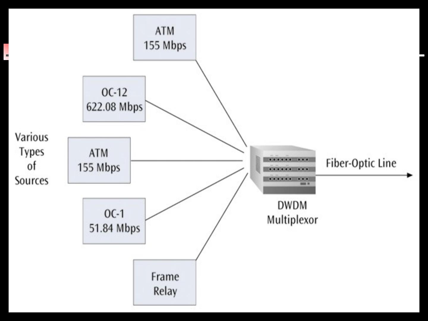
11 .Wavelength Division Multiplexing Wavelength division multiplexing multiplexes multiple data streams onto a single fiber optic line. Different wavelength lasers (called lambdas) transmit the multiple signals. Each signal carried on the fiber can be transmitted at a different rate from the other signals. Dense wavelength division multiplexing combines many (30, 40, 50, 60, more?) onto one fiber Coarse wavelength division multiplexing combines only a few lambdas

12 .12

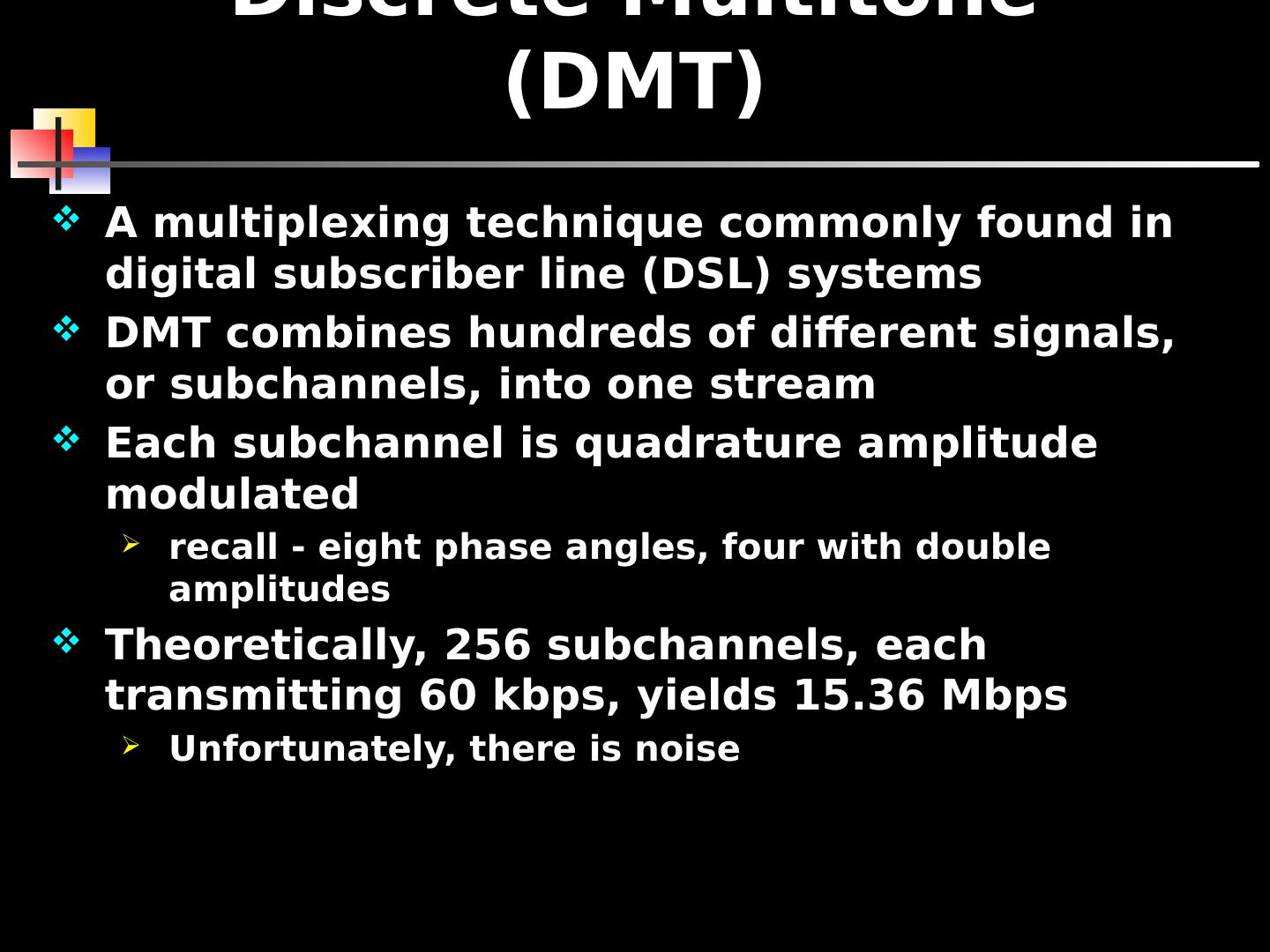
13 .Discrete Multitone (DMT) A multiplexing technique commonly found in digital subscriber line (DSL) systems DMT combines hundreds of different signals, or subchannels, into one stream Each subchannel is quadrature amplitude modulated recall - eight phase angles, four with double amplitudes Theoretically, 256 subchannels, each transmitting 60 kbps, yields 15.36 Mbps Unfortunately, there is noise

14 .14

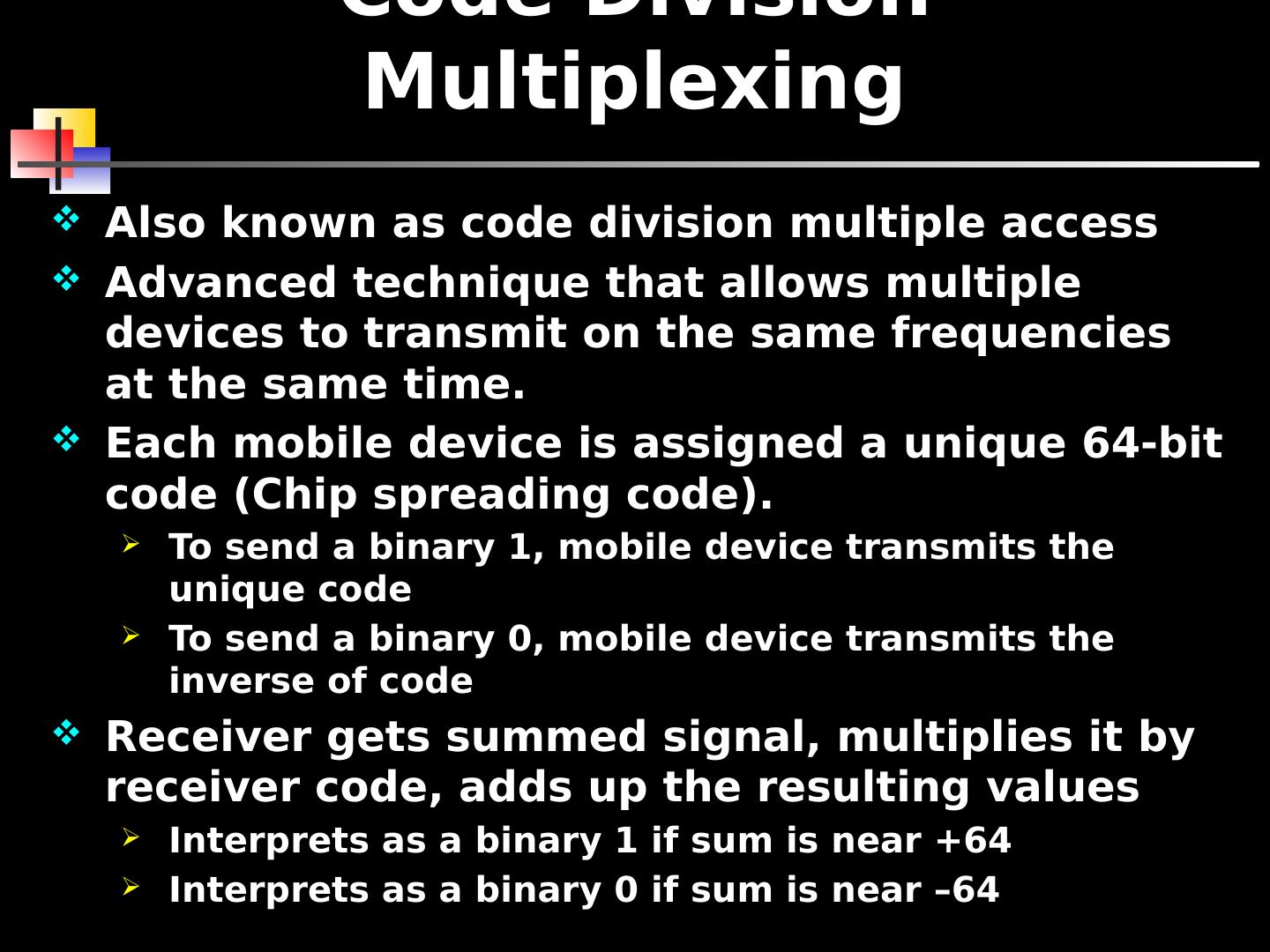
15 .Code Division Multiplexing Also known as code division multiple access Advanced technique that allows multiple devices to transmit on the same frequencies at the same time. Each mobile device is assigned a unique 64-bit code (Chip spreading code). To send a binary 1, mobile device transmits the unique code To send a binary 0, mobile device transmits the inverse of code Receiver gets summed signal, multiplies it by receiver code, adds up the resulting values Interprets as a binary 1 if sum is near +64 Interprets as a binary 0 if sum is near –64

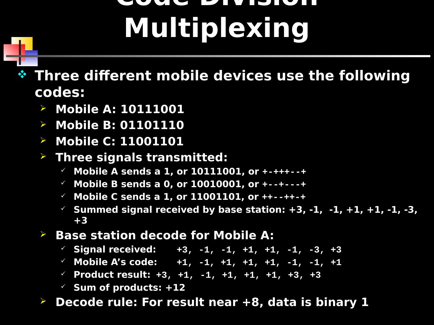
16 .Code Division Multiplexing Three different mobile devices use the following codes: Mobile A: 10111001 Mobile B: 01101110 Mobile C: 11001101 Three signals transmitted: Mobile A sends a 1, or 10111001, or +-+++--+ Mobile B sends a 0, or 10010001, or +--+---+ Mobile C sends a 1, or 11001101, or ++--++-+ Summed signal received by base station: +3, -1, -1, +1, +1, -1, -3, +3 Base station decode for Mobile A: Signal received: +3, -1, -1, +1, +1, -1, -3, +3 Mobile A’s code: +1, -1, +1, +1, +1, -1, -1, +1 Product result: +3, +1, -1, +1, +1, +1, +3, +3 Sum of products: +12 Decode rule: For result near +8, data is binary 1

17 .17

18 .Compression Compression is another technique used to squeeze more data over a communications line If you can compress a data file down to one half of its original size, file will obviously transfer in less time Two basic groups of compression: L ossless – when data is uncompressed, original data returns (Compress a financial file) Examples of lossless compression include: Huffman codes, run-length compression, and Lempel-Ziv compression Lossy – when data is uncompressed, you do not have the original data (Compress a video image, movie, or audio file) Examples of lossy compression include: MPEG, JPEG, MP3

19 .Lossless Compression Run-length encoding Replaces runs of 0s with a count of how many 0s. 000000000000001000000000110000000000000000000010…01100000000000 ^ (30 0s) 14 9 0 20 30 0 11 Replace each decimal value with a 4-bit binary value (nibble) Note: If you need to code a value larger than 15, you need to use two consecutive 4-bit nibbles The first is decimal 15, or binary 1111, and the second nibble is the remainder For example, if the decimal value is 20, you would code 1111 0101 which is equivalent to 15 + 5 If you want to code the value 15, you still need two nibbles: 1111 0000 The rule is that if you ever have a nibble of 1111, you must follow it with another nibble

20 .Lossy Compression Relative or differential encoding Video does not compress well using run-length encoding In one color video frame, not much is alike But what about from frame to frame? Send a frame, store it in a buffer Next frame is just difference from previous frame Then store that frame in buffer, etc. 5 7 6 2 8 6 6 3 5 6 6 5 7 5 5 6 3 2 4 7 8 4 6 8 5 6 4 8 8 5 5 1 2 9 8 6 5 5 6 6 First Frame 5 7 6 2 8 6 6 3 5 6 6 5 7 6 5 6 3 2 3 7 8 4 6 8 5 6 4 8 8 5 5 1 3 9 8 6 5 5 7 6 Second Frame 0 0 0 0 0 0 0 0 0 0 0 0 0 1 0 0 0 0 -1 0 0 0 0 0 0 0 0 0 0 0 0 0 1 0 0 0 0 0 1 0 Difference

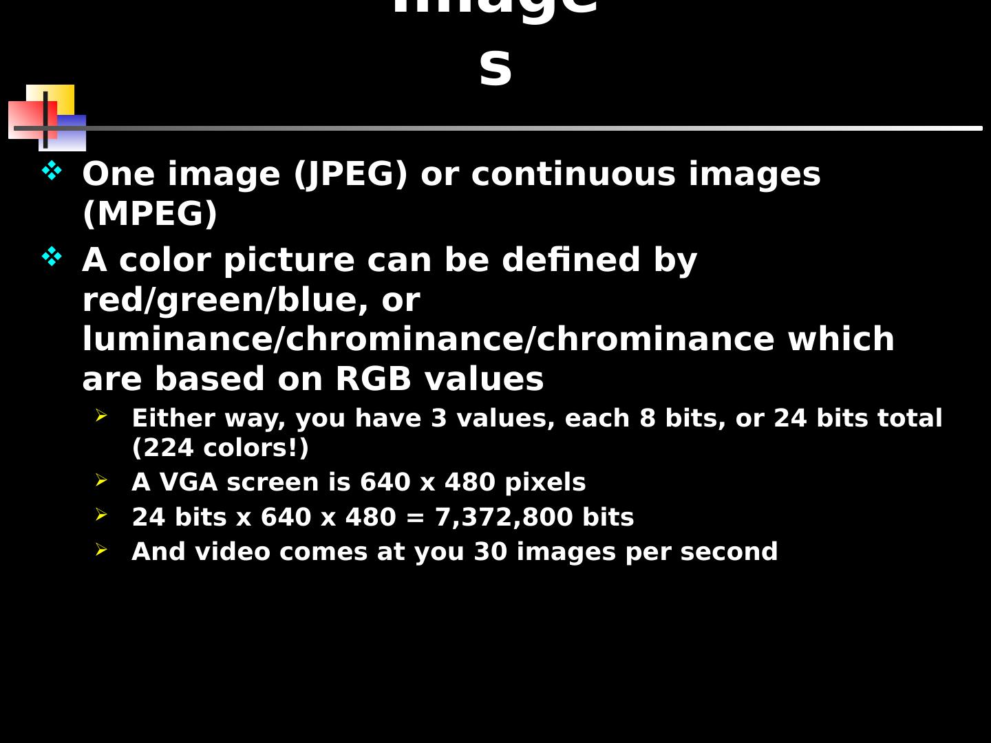
21 .Images One image (JPEG) or continuous images (MPEG) A color picture can be defined by red/green/blue, or luminance/chrominance/chrominance which are based on RGB values Either way, you have 3 values, each 8 bits, or 24 bits total (224 colors!) A VGA screen is 640 x 480 pixels 24 bits x 640 x 480 = 7,372,800 bits And video comes at you 30 images per second

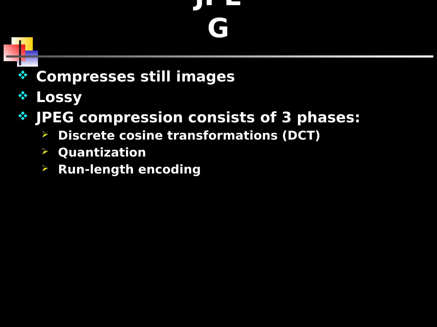
22 .JPEG Compresses still images Lossy JPEG compression consists of 3 phases: Discrete cosine transformations (DCT) Quantization Run-length encoding

23 .JPEG - DCT Divide image into a series of 8x8 pixel blocks If the original image was 640x480 pixels, the new picture would be 80 blocks x 60 blocks If B&W, each pixel in 8x8 block is an 8-bit value (0-255) If color, each pixel is a 24-bit value (8 bits for red, 8 bits for blue, and 8 bits for green) Takes an 8x8 array (P) and produces a new 8x8 array (T) using cosines T matrix contains a collection of values called spatial frequencies These spatial frequencies relate directly to how much the pixel values change as a function of their positions in the block An image with uniform color changes (little fine detail) has a P array with closely similar values and a corresponding T array with many zero values An image with large color changes over a small area (lots of fine detail) has a P array with widely changing values, and thus a T array with many non-zero values

24 .JPEG - Quantization The human eye can’t see small differences in color So take T matrix and divide all values by 10 Will give us more zero entries More 0s means more compression! But this is too lossy And dividing all values by 10 doesn’t take into account that upper left of matrix has more action (the less subtle features of the image, or low spatial frequencies)

25 .80 blocks 60 blocks 640 x 480 VGA Screen Image Divided into 8 x 8 Pixel Blocks 25

26 .DCT Quantization U matrix 26

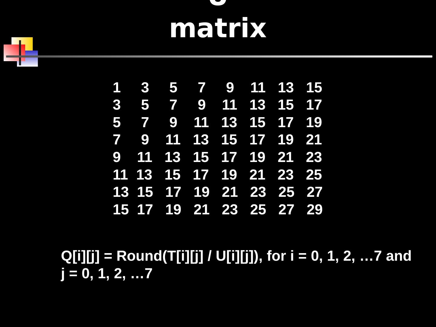
27 .U matrix 1 3 5 7 9 11 13 15 3 5 7 9 11 13 15 17 5 7 9 11 13 15 17 19 7 9 11 13 15 17 19 21 9 11 13 15 17 19 21 23 11 13 15 17 19 21 23 25 13 15 17 19 21 23 25 27 15 17 19 21 23 25 27 29 Q[i][j] = Round(T[i][j] / U[i][j]), for i = 0, 1, 2, …7 and j = 0, 1, 2, …7

28 .JPEG - Run-length encoding Now take the quantized matrix Q and perform run-length encoding on it But don’t just go across the rows Longer runs of zeros if you perform the run-length encoding in a diagonal fashion

29 .JPEG Uncompress Undo run-length encoding Multiply matrix Q by matrix U yielding matrix T Apply similar cosine calculations to get original P matrix back