对极几何和立体视觉

1 .Epipolar Geometry and Stereo Vision Computer Vision Jia-Bin Huang, Virginia Tech Many slides from S. Seitz and D. Hoiem

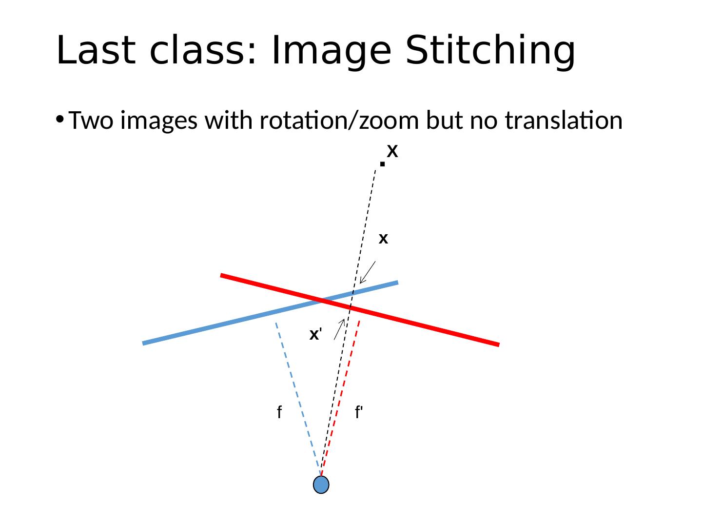
2 .Last class: Image Stitching Two images with rotation/zoom but no translation f f . x x X

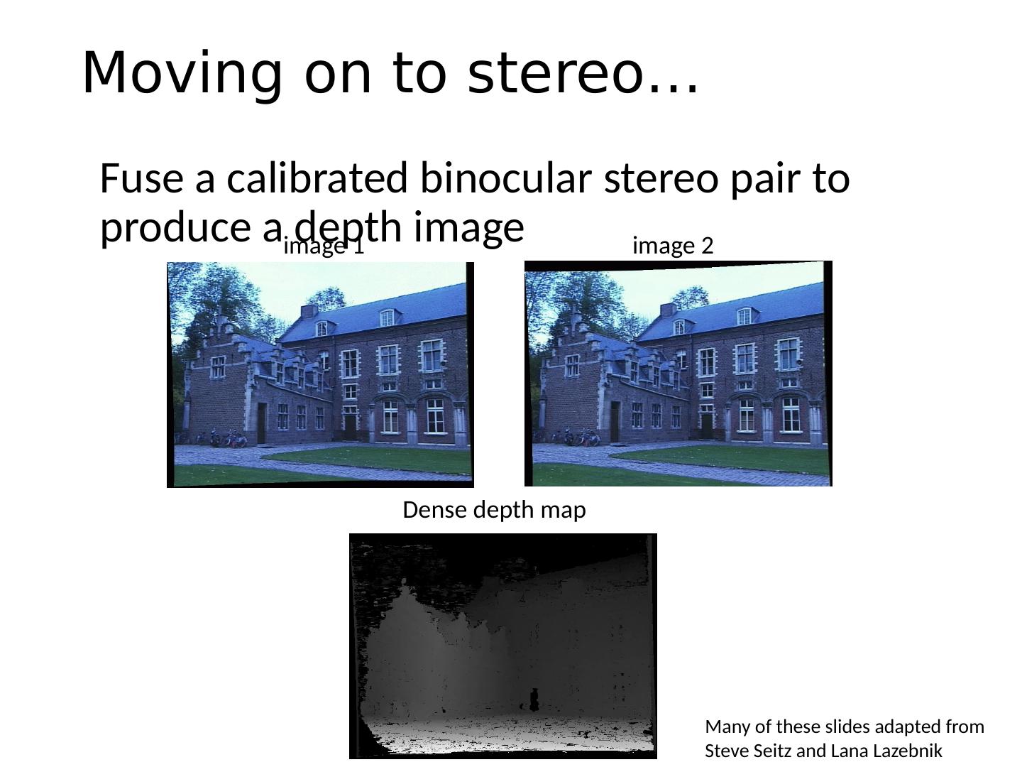
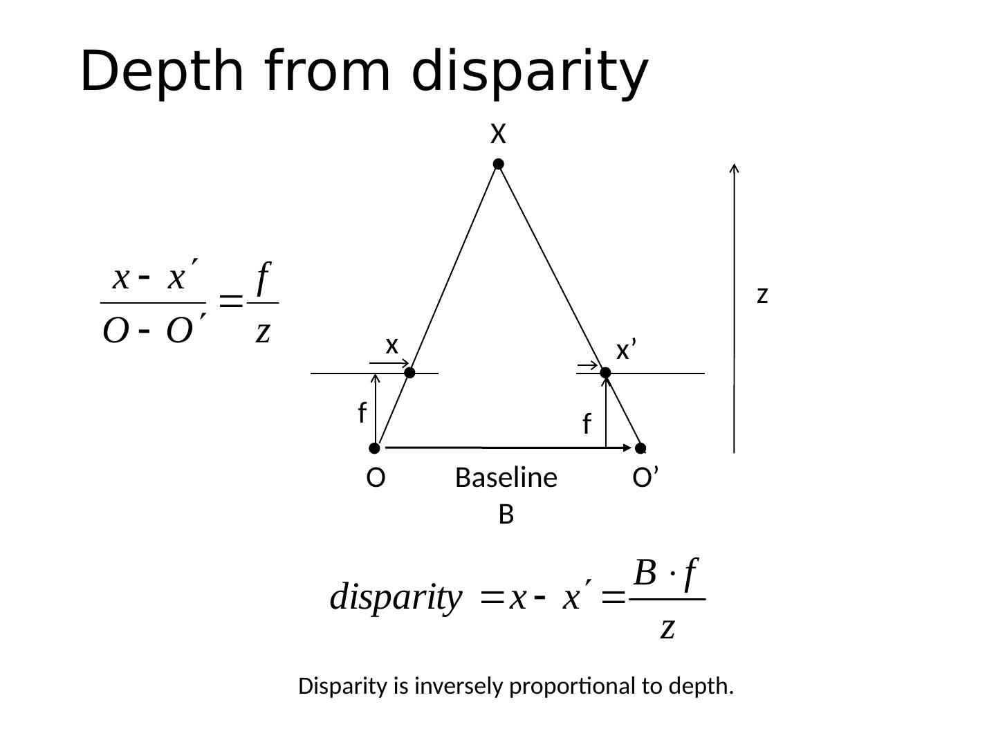
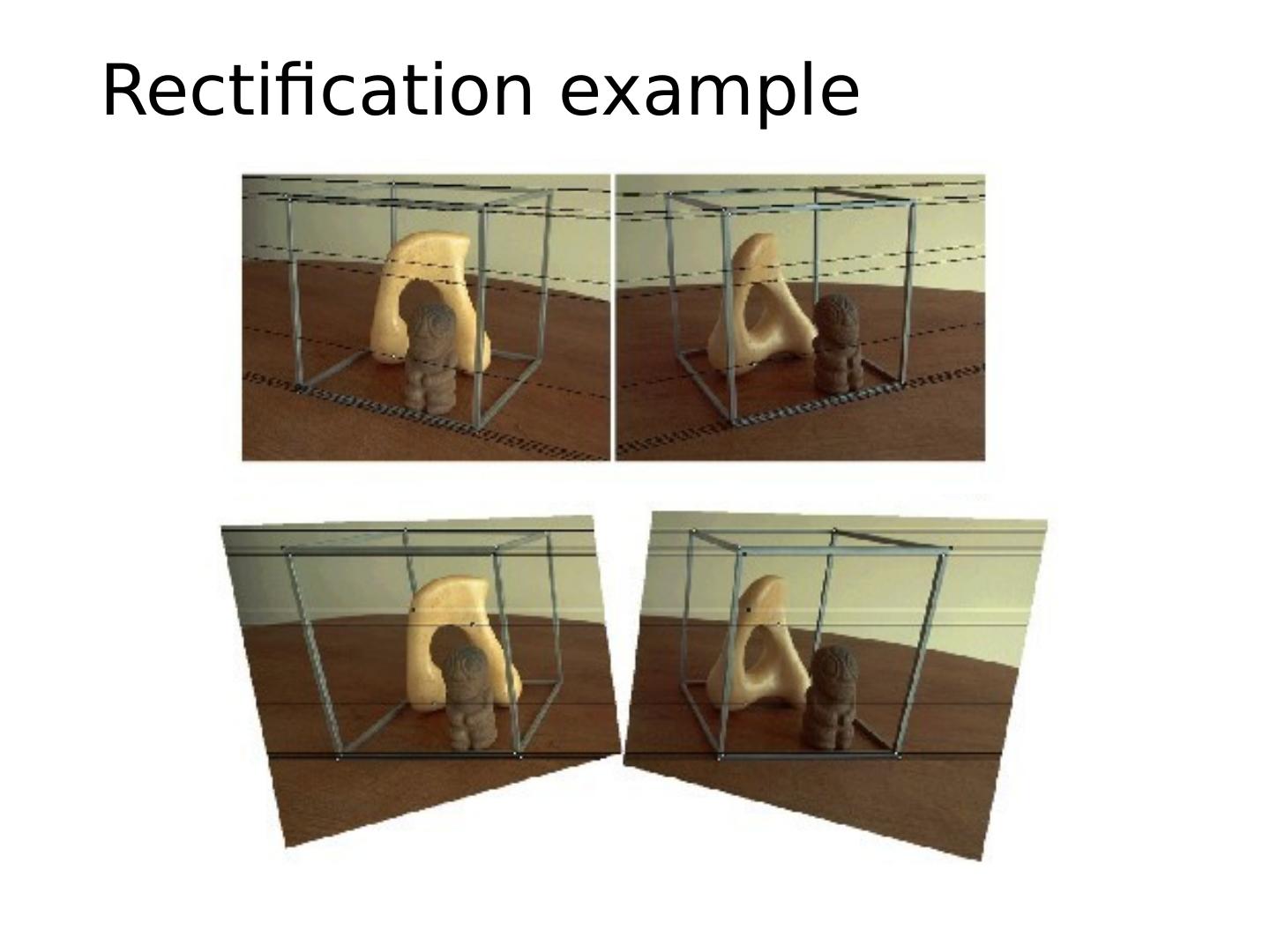
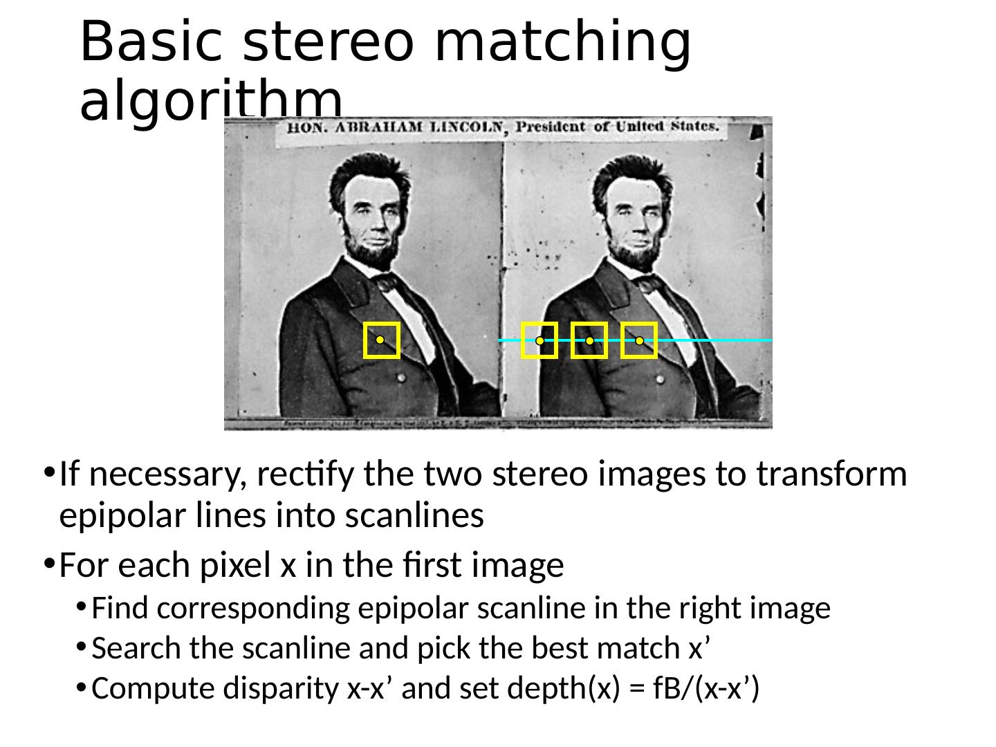
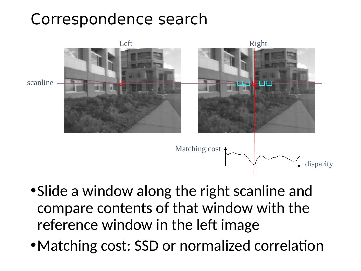
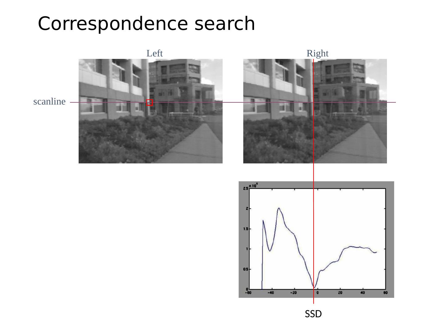
3 .This class: Two-View Geometry Epipolar geometry Relates cameras from two positions Stereo depth estimation Recover depth from two images

4 .This class: Two-View Geometry Epipolar geometry Relates cameras from two positions Stereo depth estimation Recover depth from two images

5 .This class: Two-View Geometry Epipolar geometry Relates cameras from two positions Stereo depth estimation Recover depth from two images

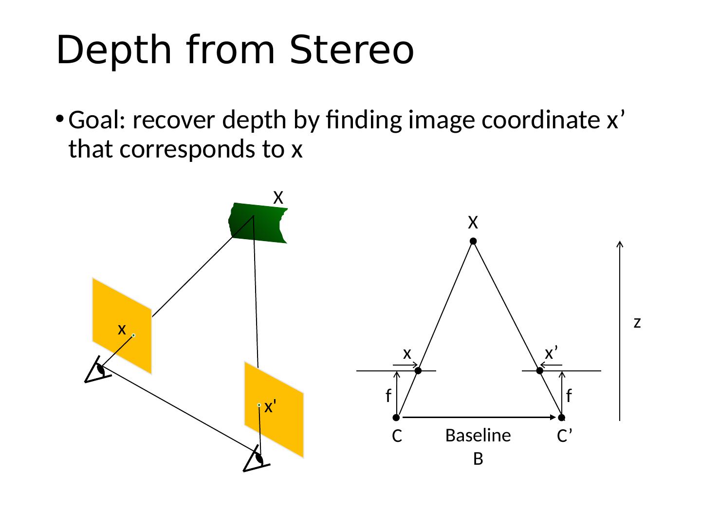
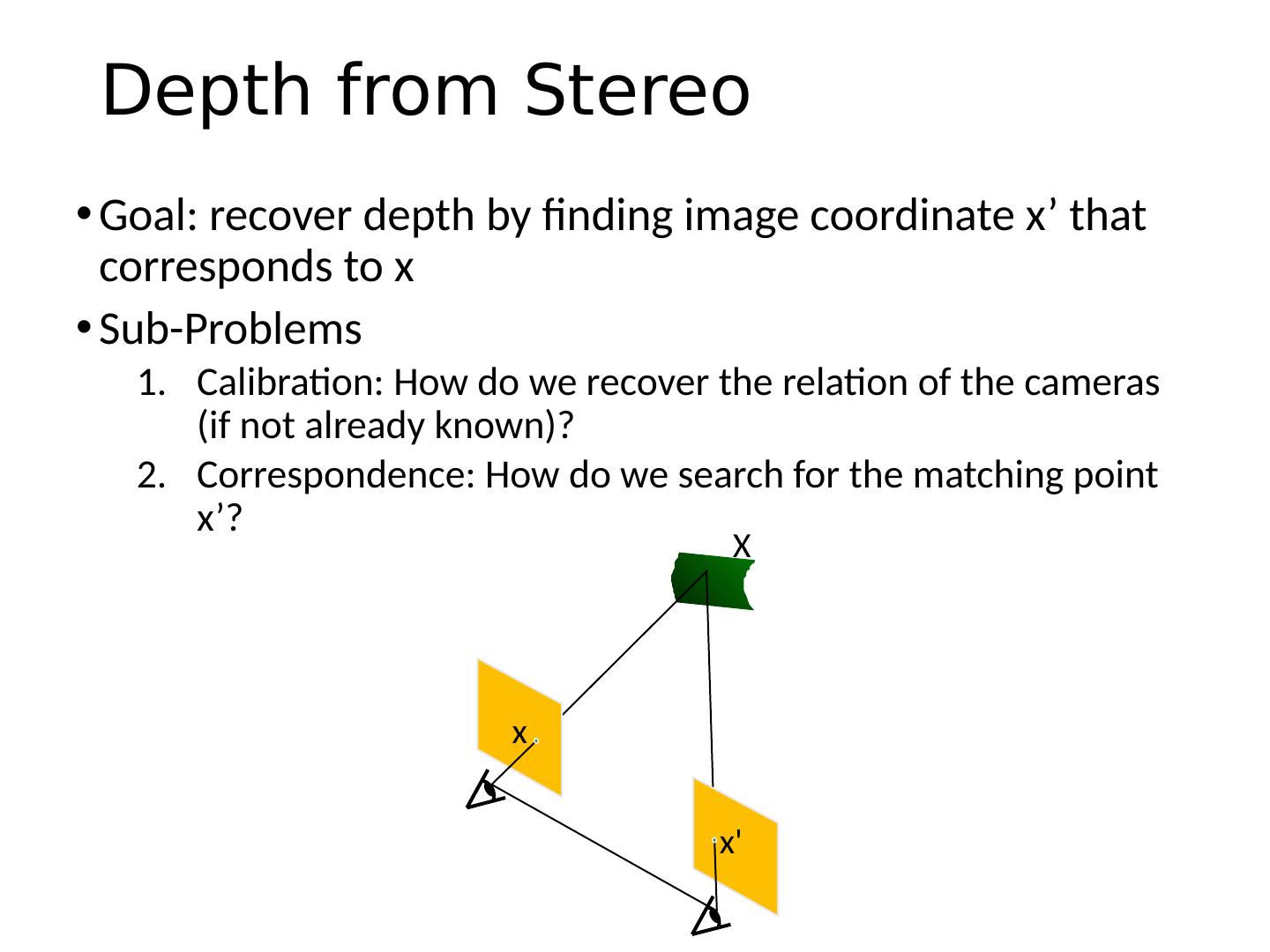
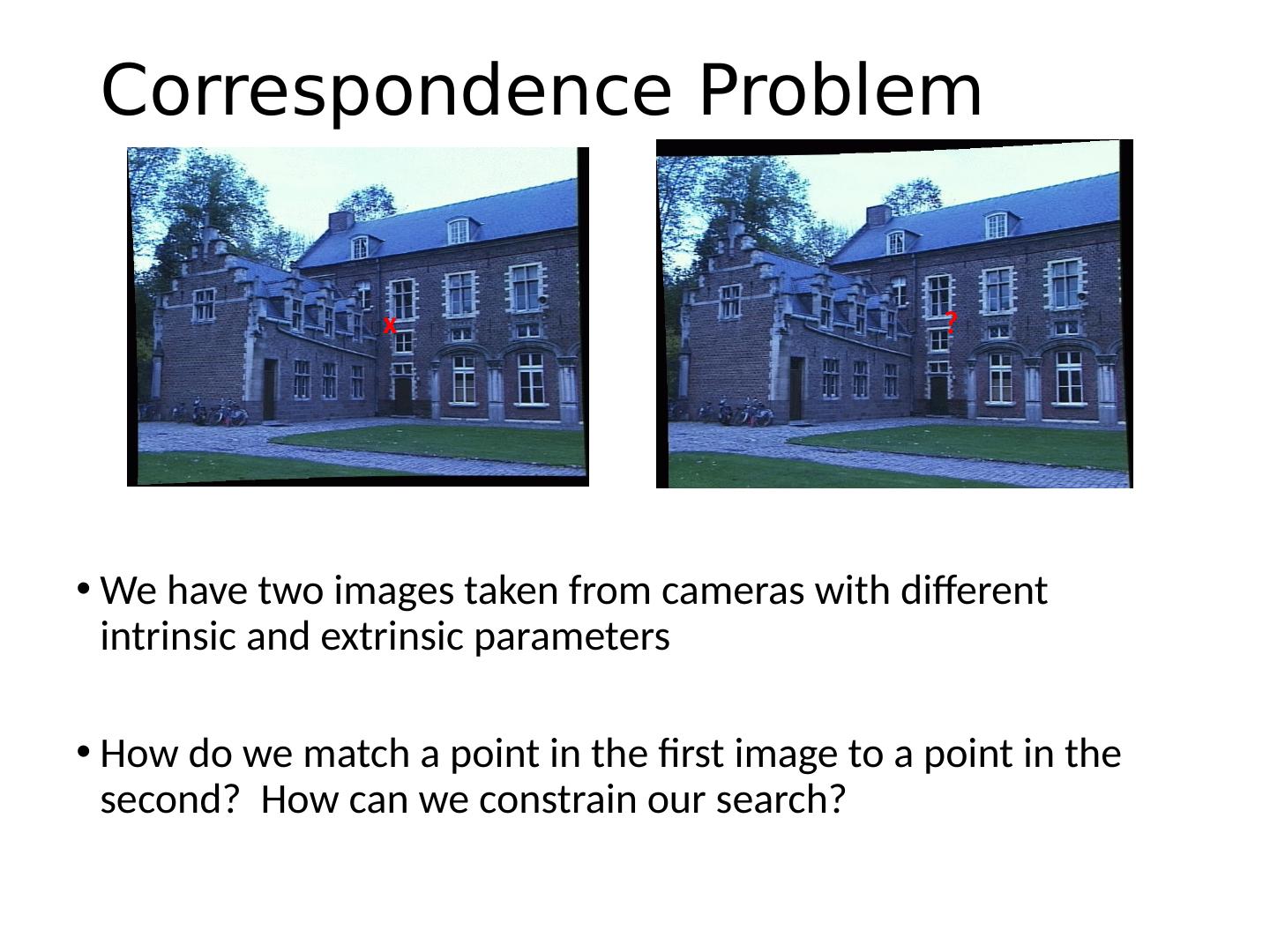
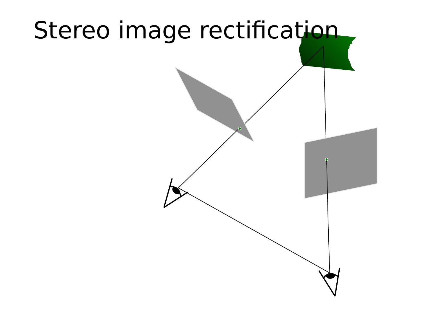
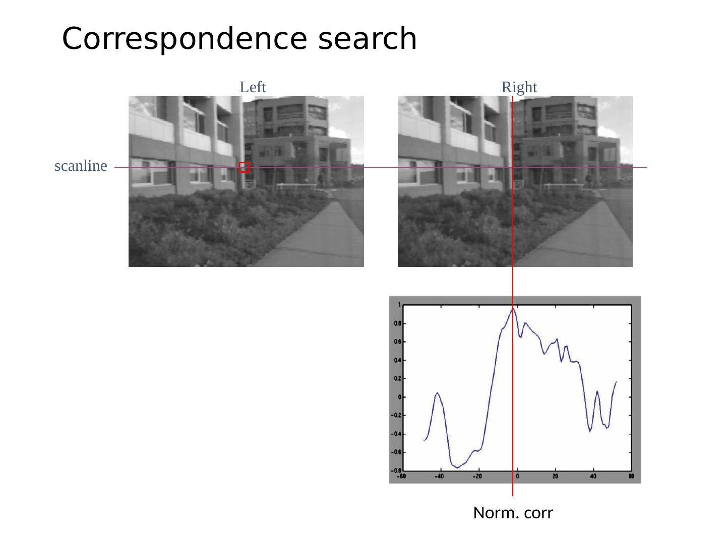
6 .Correspondence Problem We have two images taken from cameras with different intrinsic and extrinsic parameters How do we match a point in the first image to a point in the second? How can we constrain our search? x ?

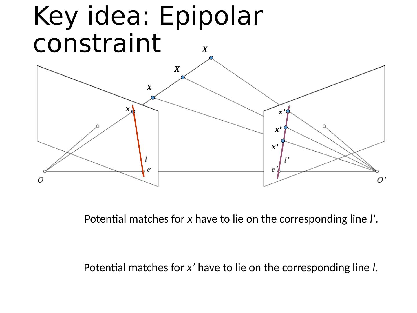
7 .Key idea: Epipolar constraint

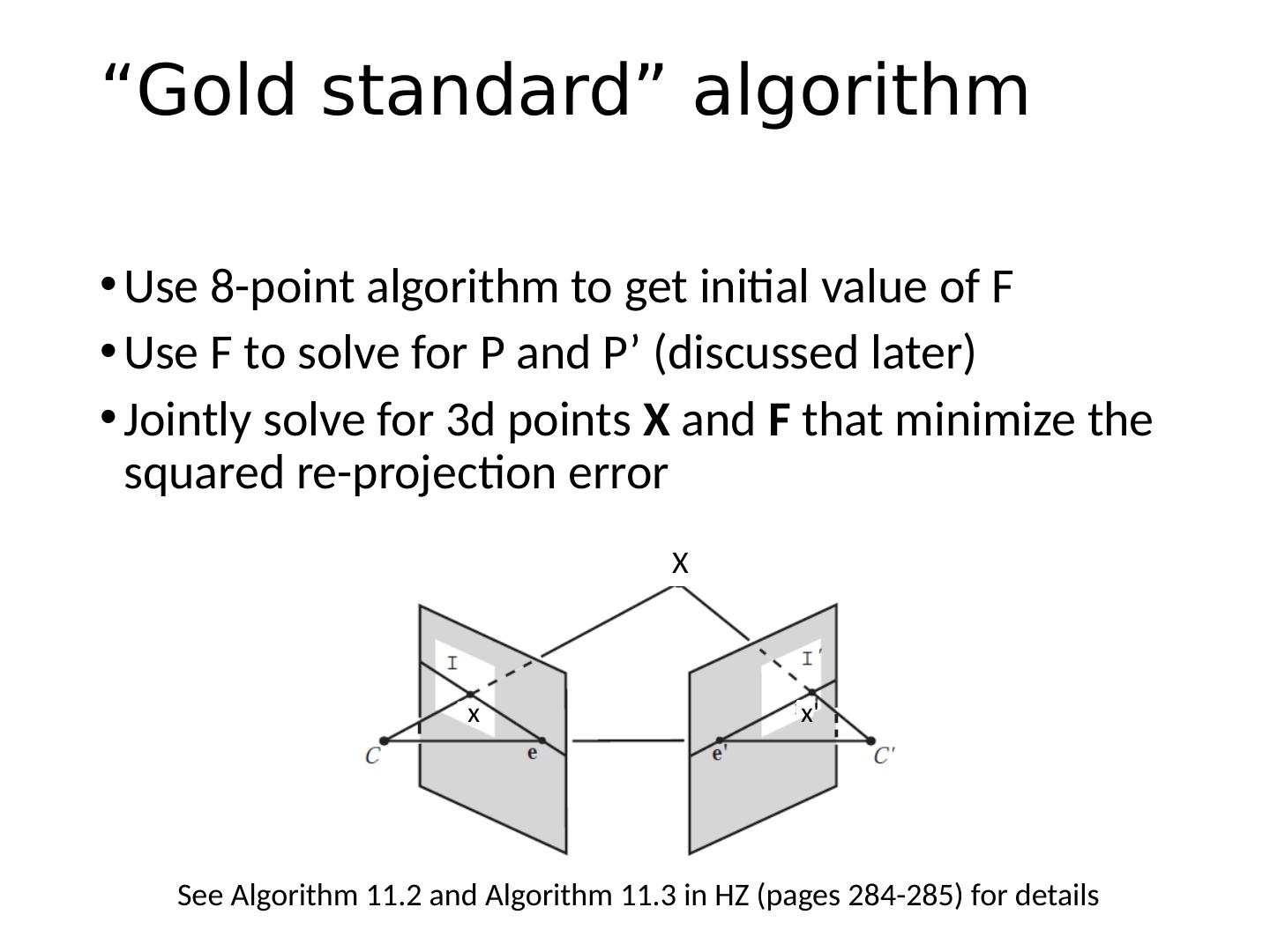
8 .Potential matches for x have to lie on the corresponding line l’ . Potential matches for x’ have to lie on the corresponding line l . Key idea: Epipolar constraint x x’ X x’ X x’ X

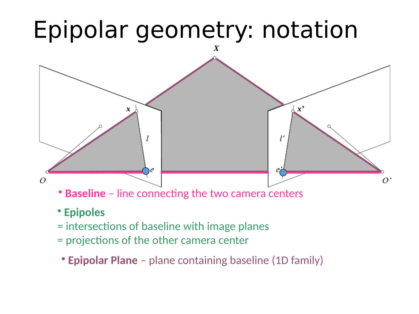
9 . Epipolar Plane – plane containing baseline (1D family) Epipoles = intersections of baseline with image planes = projections of the other camera center Baseline – line connecting the two camera centers Epipolar geometry: notation X x x’

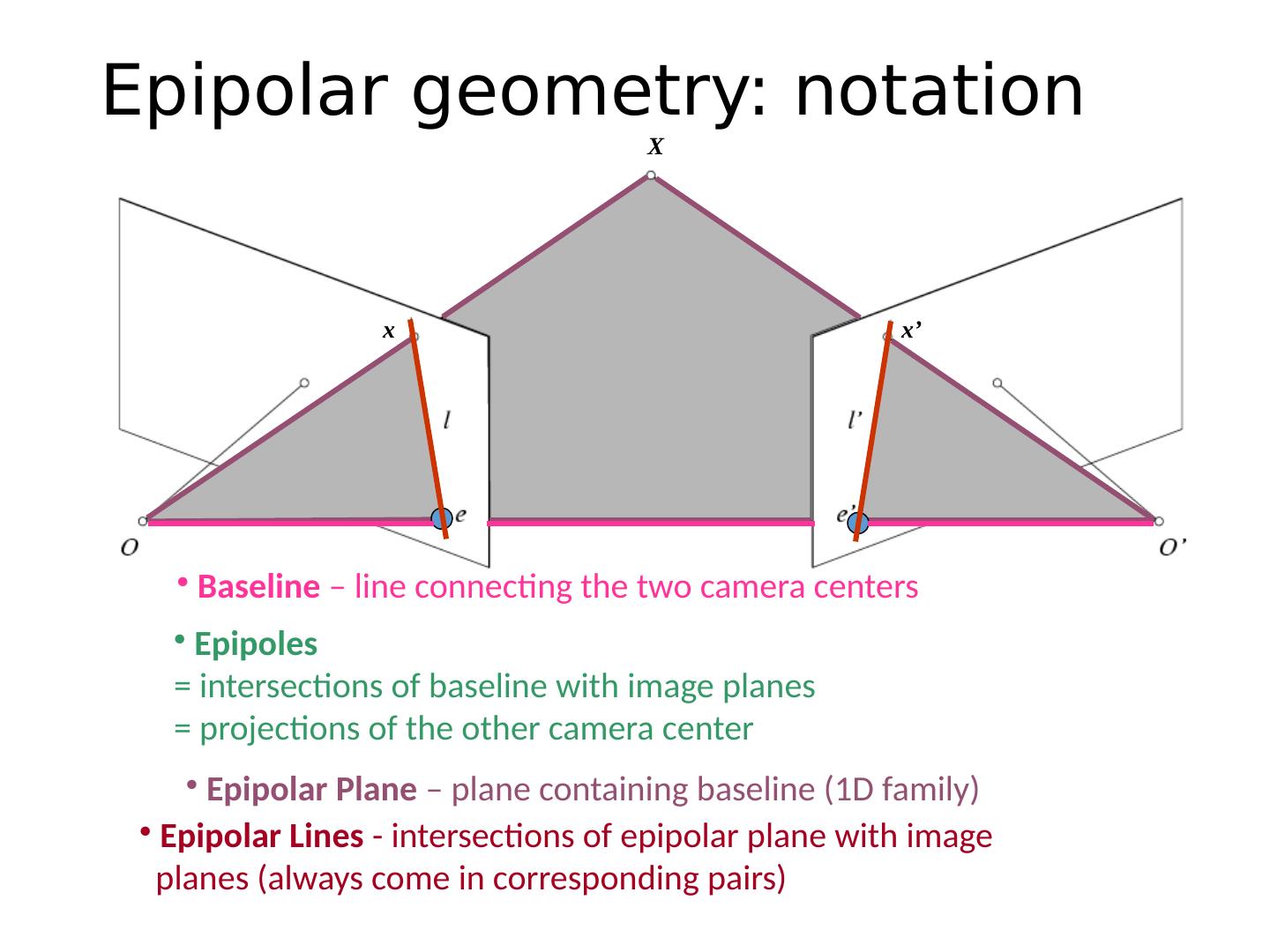
10 . Epipolar Lines - intersections of epipolar plane with image planes (always come in corresponding pairs) Epipolar geometry: notation X x x’ Epipolar Plane – plane containing baseline (1D family) Epipoles = intersections of baseline with image planes = projections of the other camera center Baseline – line connecting the two camera centers

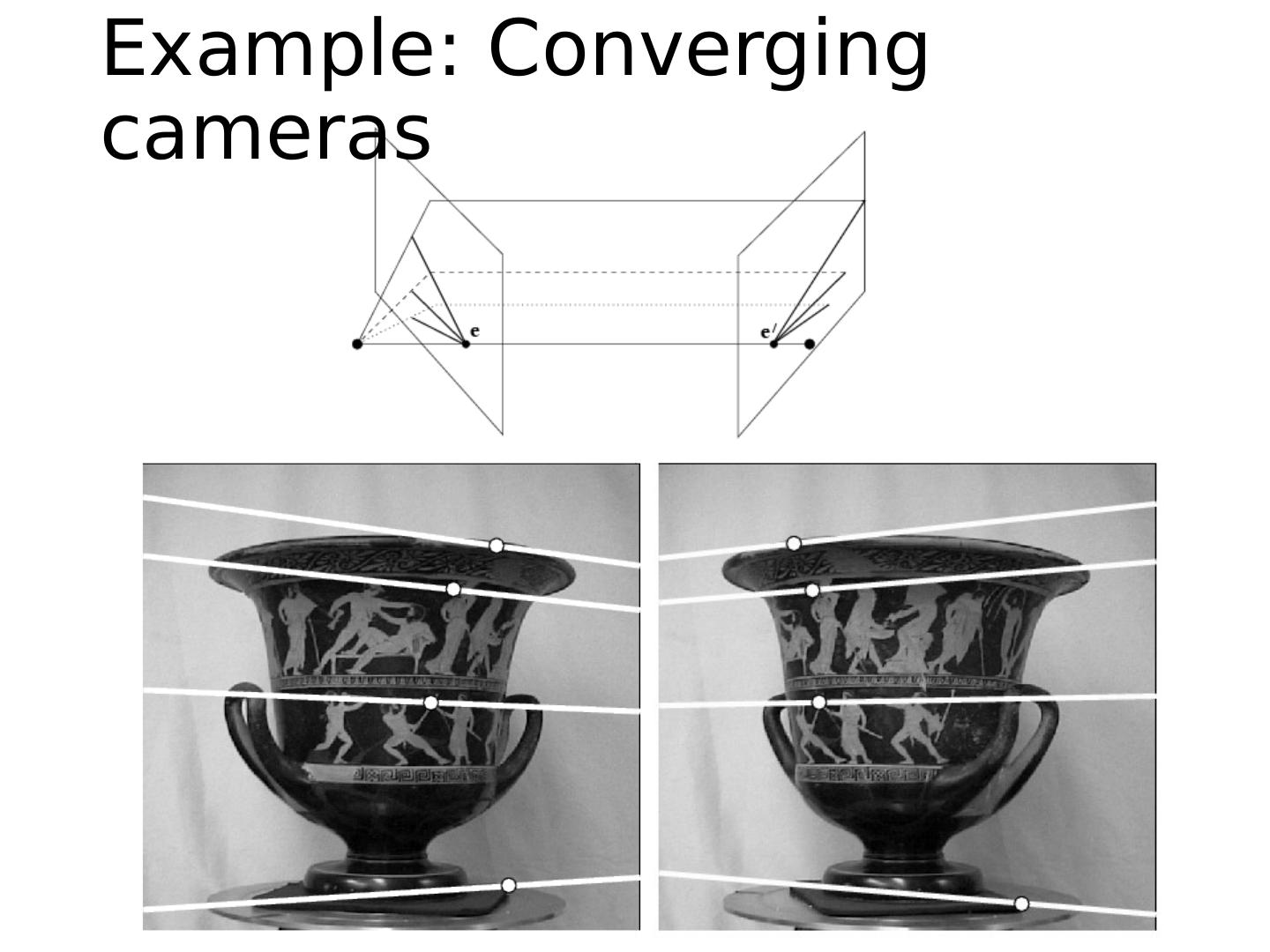
11 .Example: Converging cameras

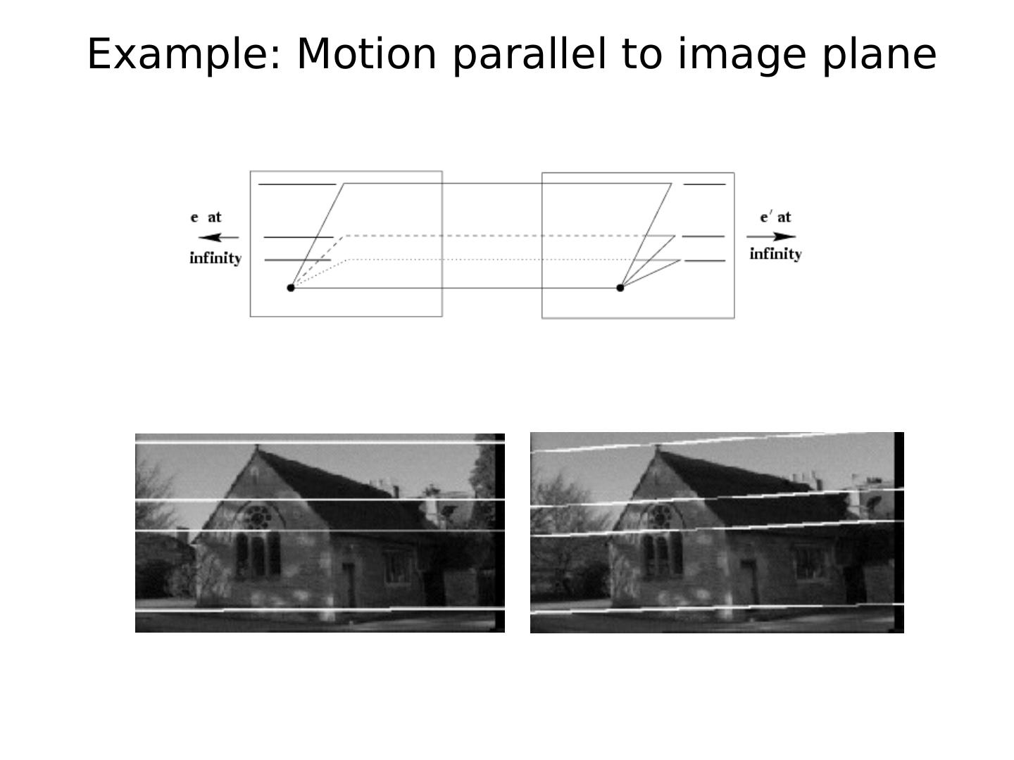
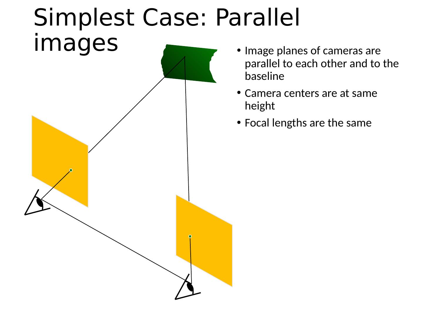
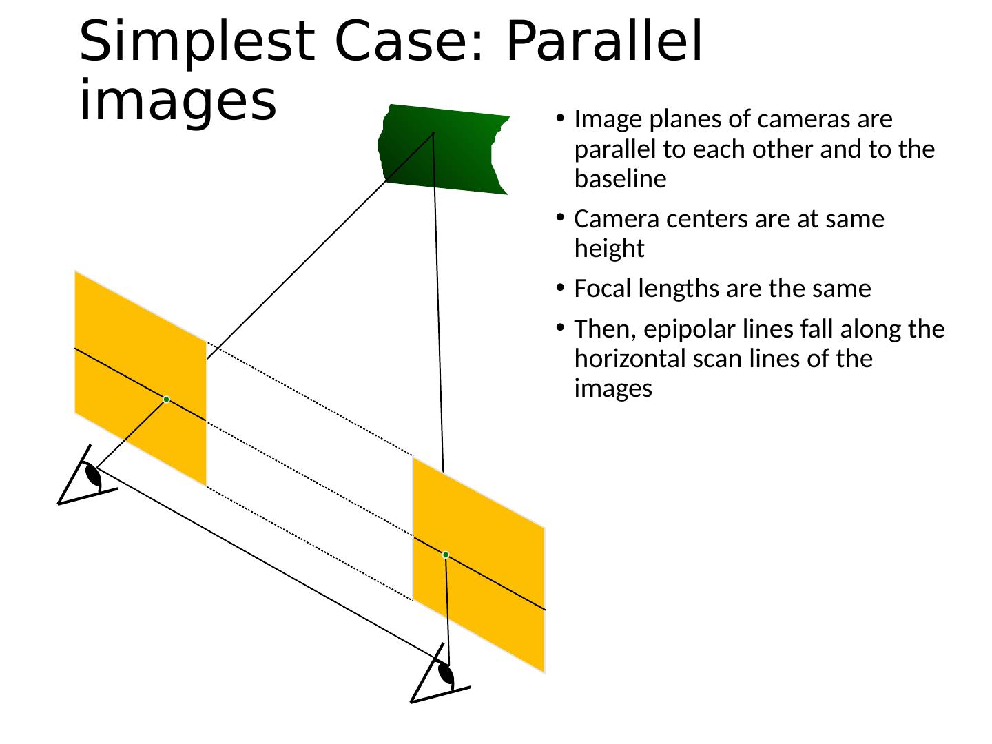
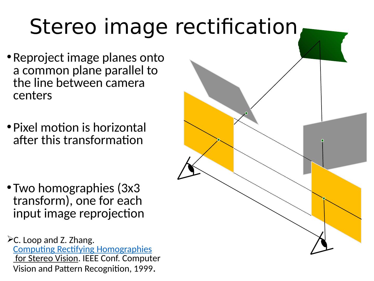
12 .Example: Motion parallel to image plane

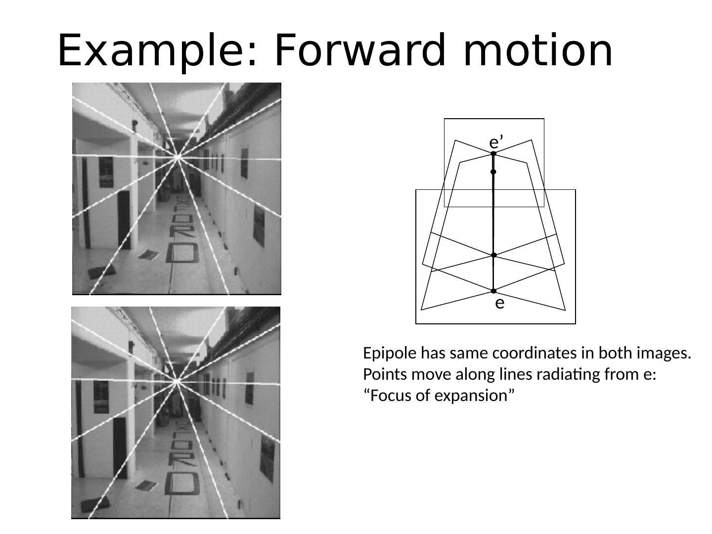
13 .Example: Forward motion What would the epipolar lines look like if the camera moves directly forward?

14 .e e’ Example: Forward motion Epipole has same coordinates in both images. Points move along lines radiating from e: “Focus of expansion”

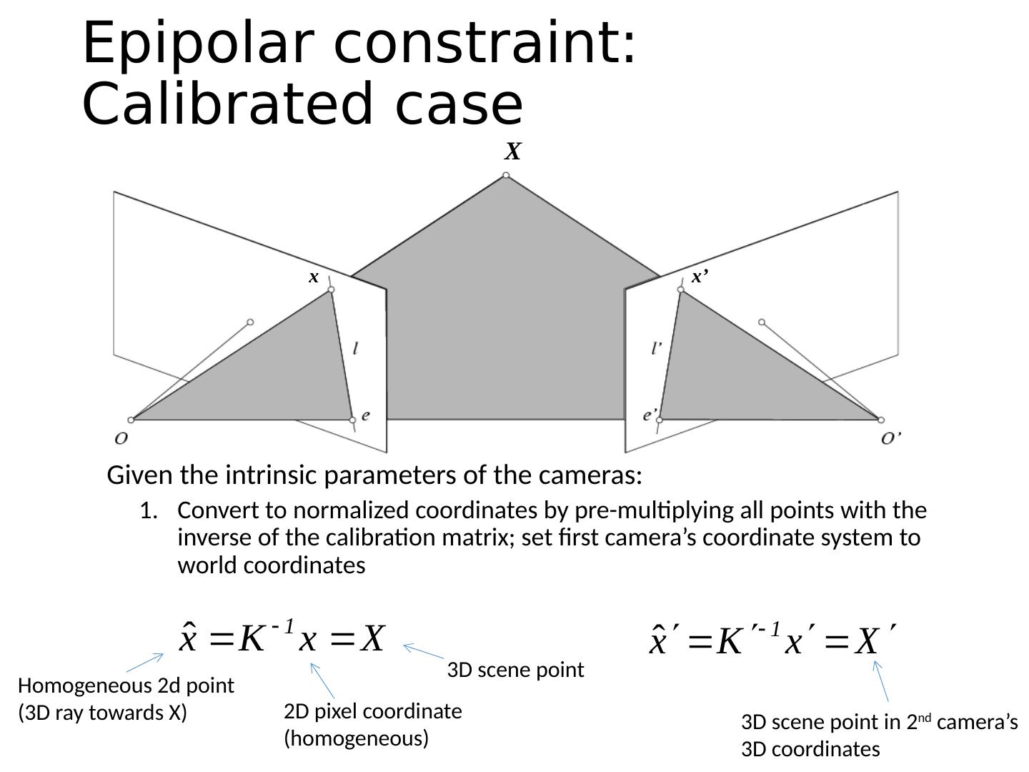
15 .X x x’ Epipolar constraint: Calibrated case Given the intrinsic parameters of the cameras : Convert to normalized coordinates by pre-multiplying all points with the inverse of the calibration matrix; set first camera’s coordinate system to world coordinates Homogeneous 2d point (3D ray towards X) 2D pixel coordinate (homogeneous) 3D scene point 3D scene point in 2 nd camera’s 3D coordinates

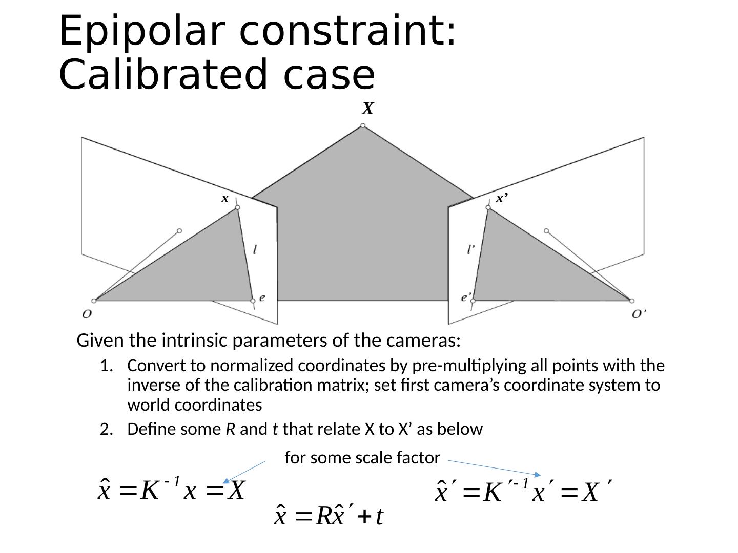
16 .X x x’ Epipolar constraint: Calibrated case Given the intrinsic parameters of the cameras: Convert to normalized coordinates by pre-multiplying all points with the inverse of the calibration matrix; set first camera’s coordinate system to world coordinates Define some R and t that relate X to X’ as below for some scale factor

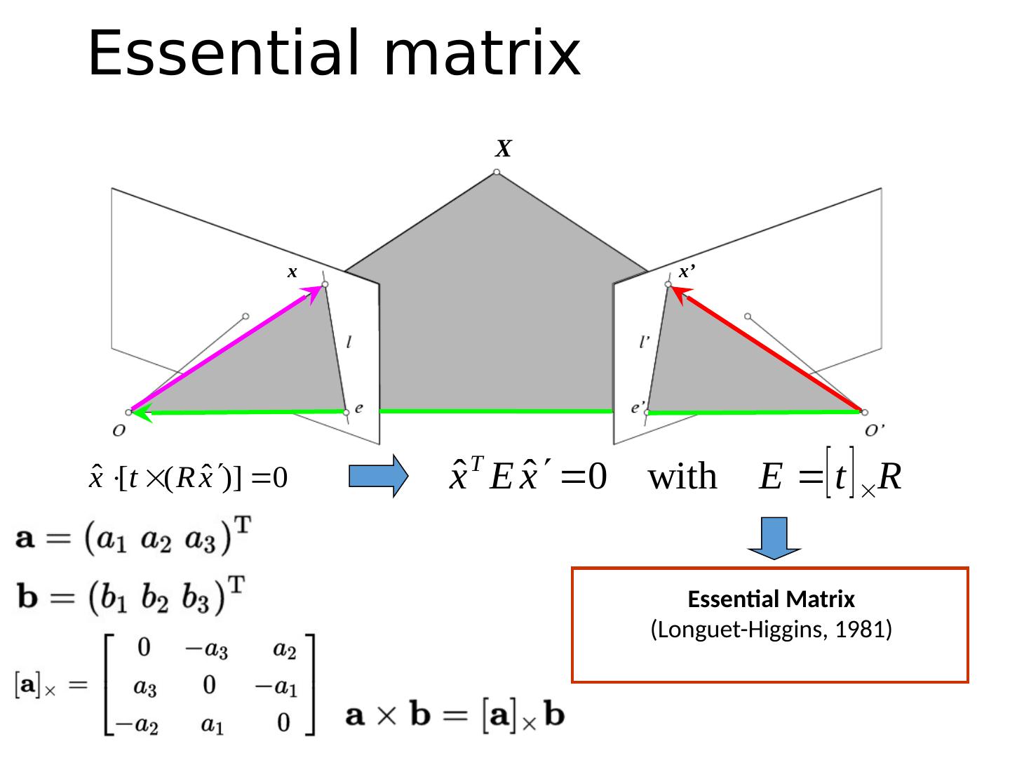
17 .Epipolar constraint: Calibrated case x x’ X (because and are co-planar)          

18 .Essential Matrix (Longuet-Higgins, 1981) Essential matrix X x x’

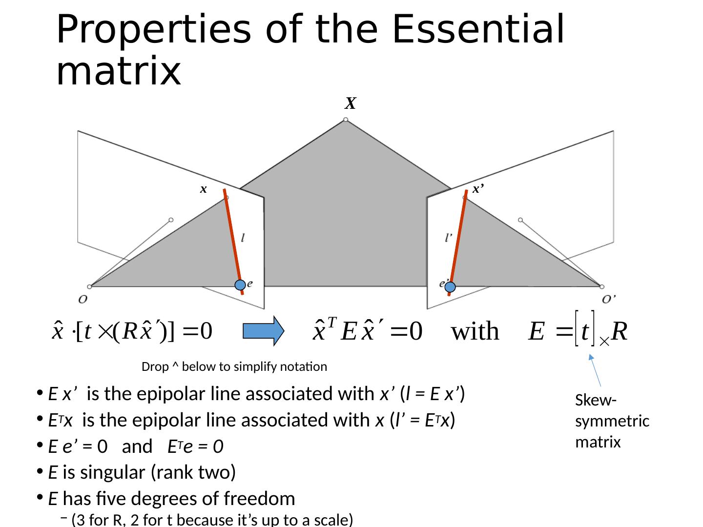
19 .X Properties of the Essential matrix E x’ is the epipolar line associated with x’ ( l = E x’ ) E T x is the epipolar line associated with x ( l’ = E T x ) E e ’ = 0 and E T e = 0 E is singular (rank two) E has five degrees of freedom (3 for R, 2 for t because it’s up to a scale) Drop ^ below to simplify notation x x’ Skew-symmetric matrix

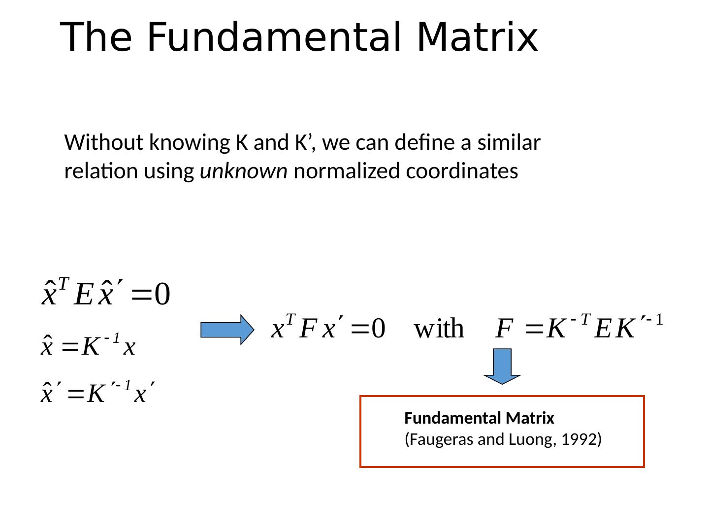
20 .Epipolar constraint: Uncalibrated case If we don’t know K and K’ , then we can write the epipolar constraint in terms of unknown normalized coordinates: X x x’

21 .The Fundamental Matrix Fundamental Matrix ( Faugeras and Luong , 1992) Without knowing K and K’, we can define a similar relation using unknown normalized coordinates

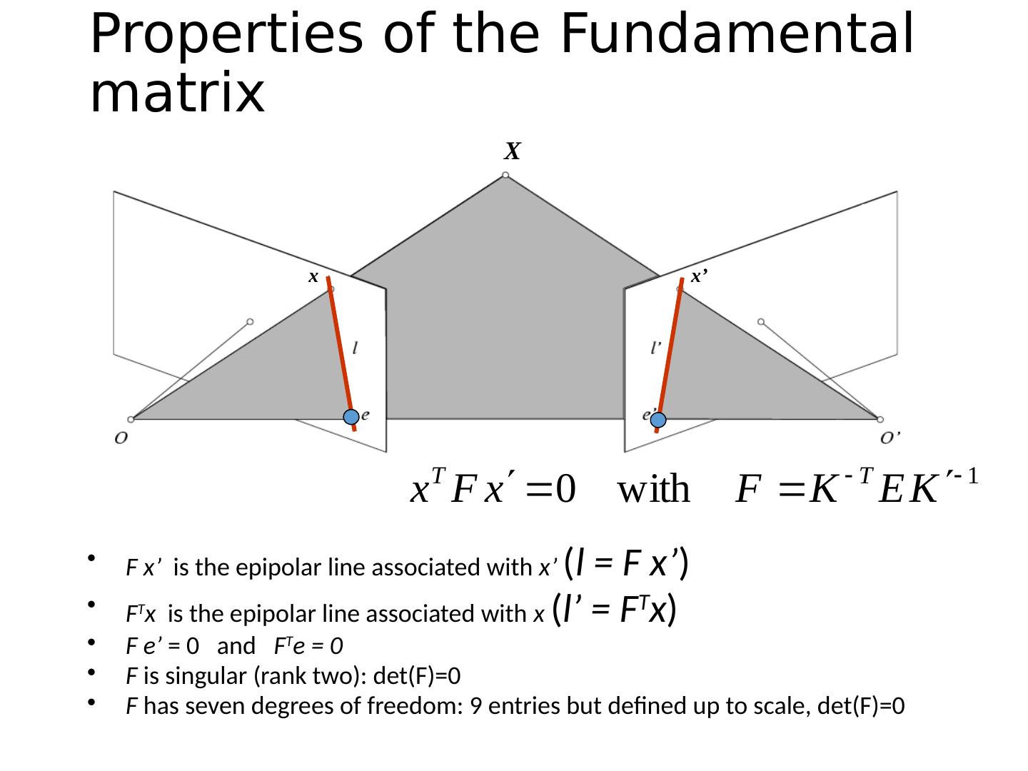
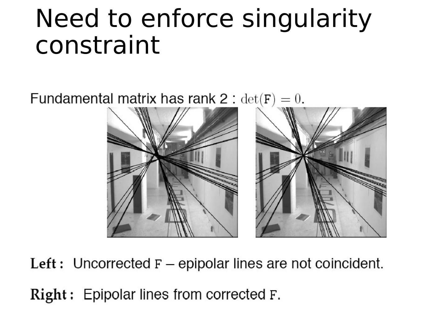
22 .Properties of the Fundamental matrix F x’ is the epipolar line associated with x’ ( l = F x’ ) F T x is the epipolar line associated with x ( l’ = F T x ) F e’ = 0 and F T e = 0 F is singular (rank two): det (F)=0 F has seven degrees of freedom: 9 entries but defined up to scale, det (F)=0 X x x’

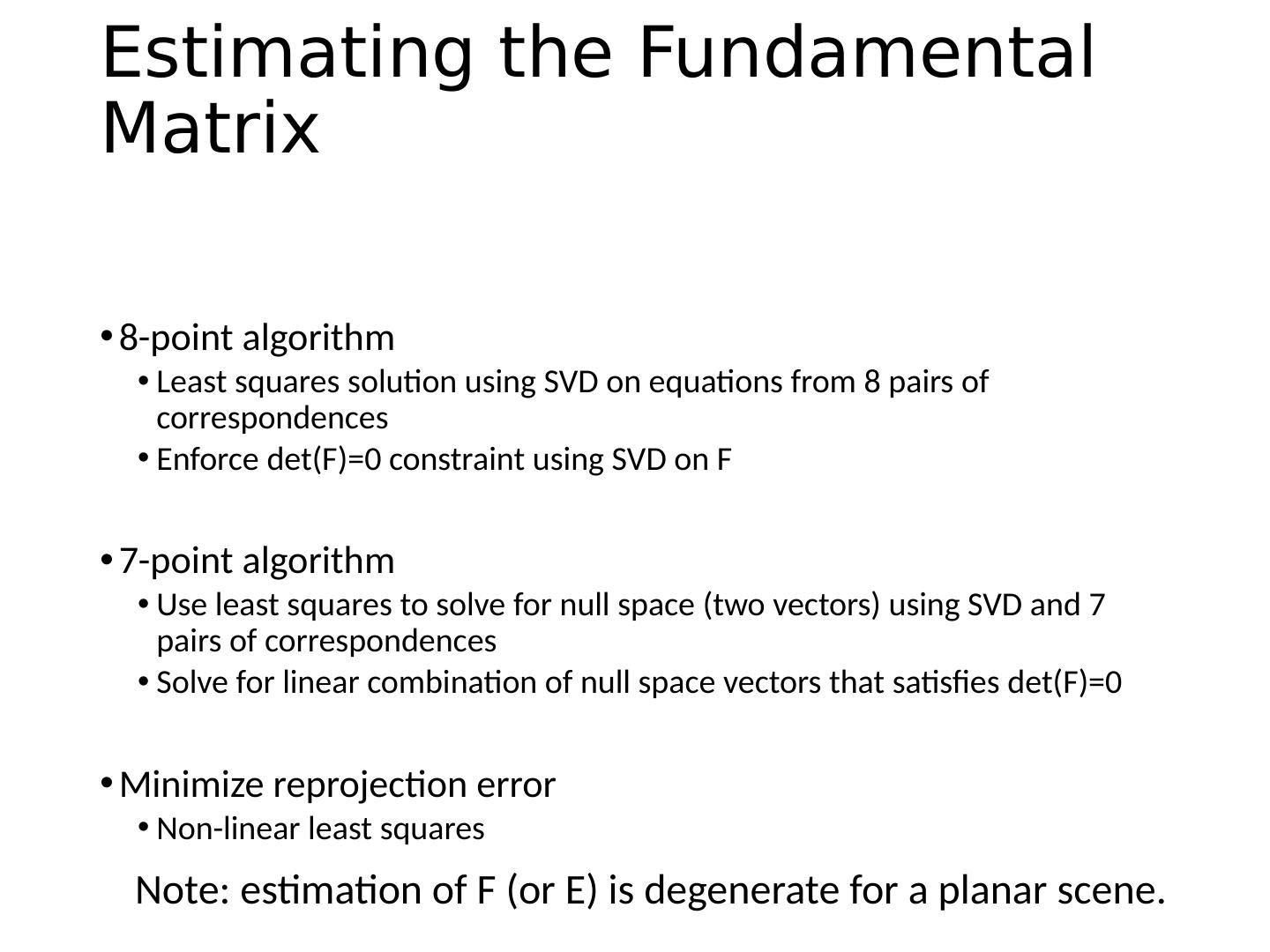
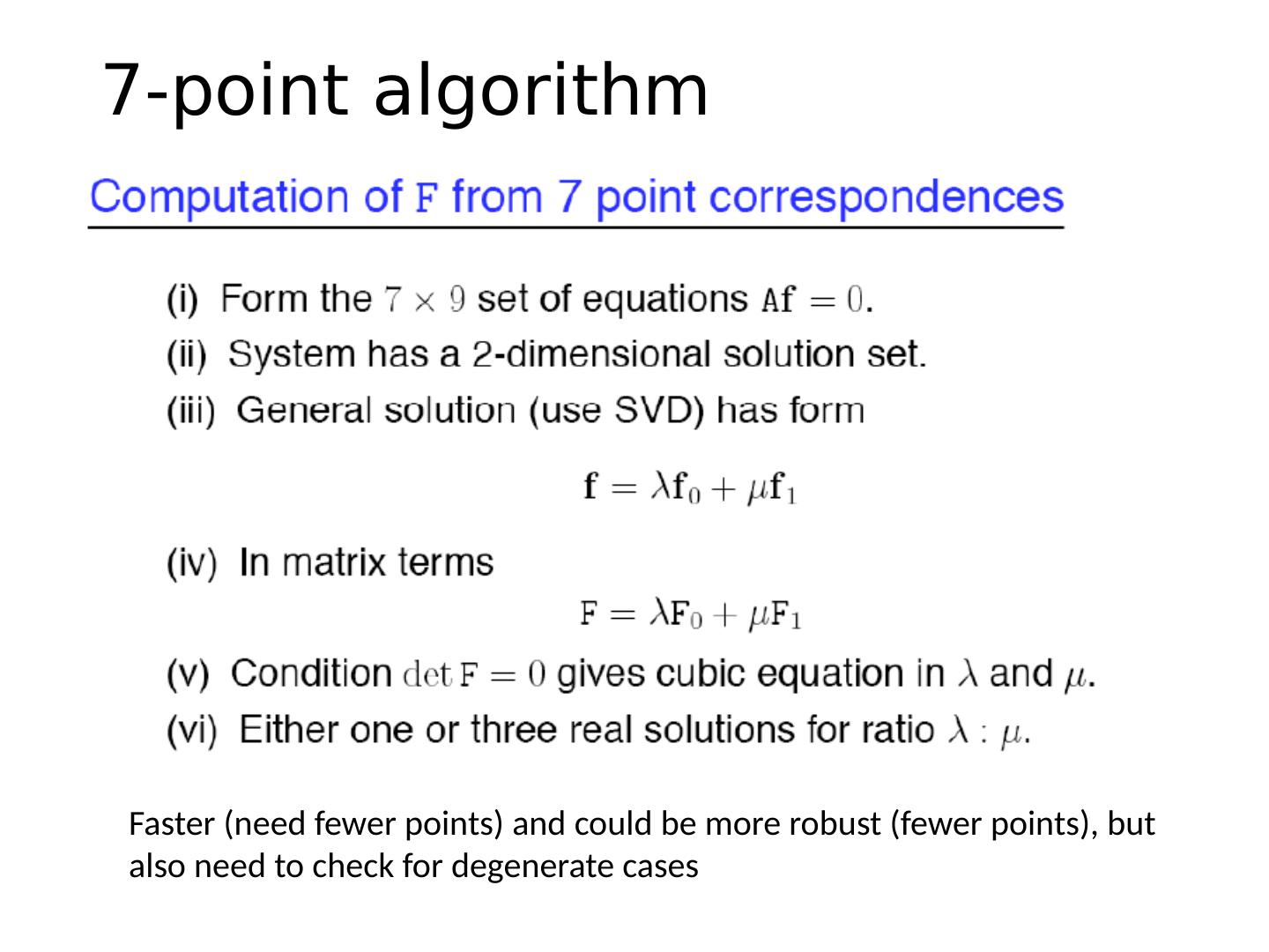
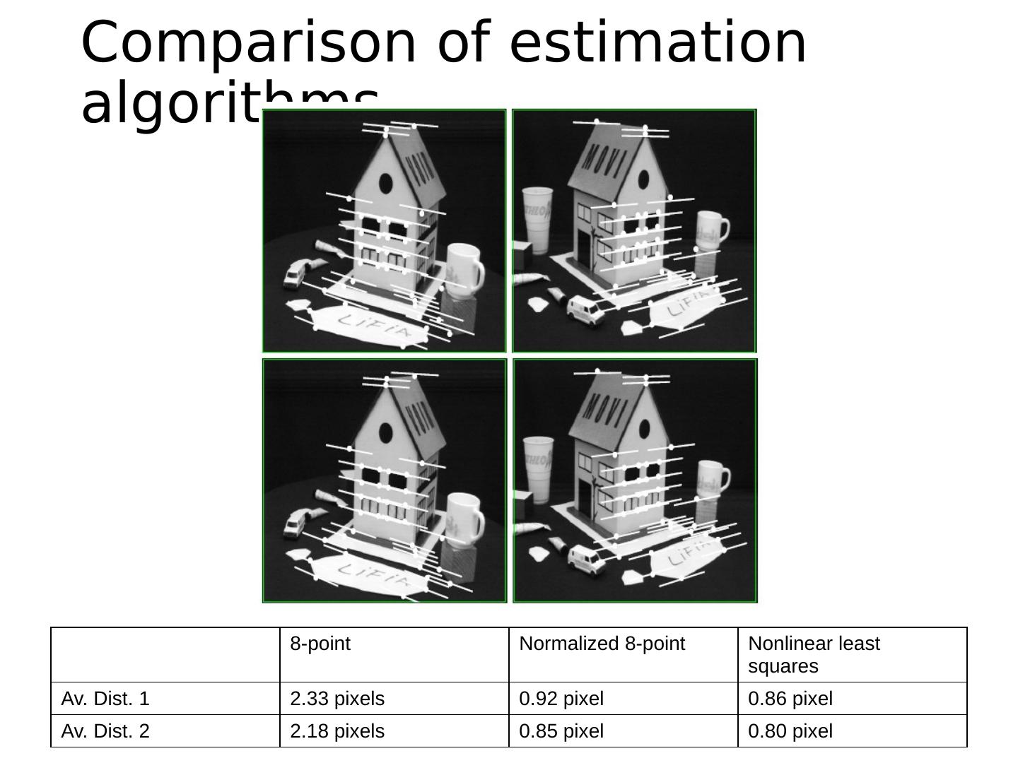
23 .Estimating the Fundamental Matrix 8-point algorithm Least squares solution using SVD on equations from 8 pairs of correspondences Enforce det (F)=0 constraint using SVD on F 7-point algorithm Use least squares to solve for null space (two vectors) using SVD and 7 pairs of correspondences Solve for linear combination of null space vectors that satisfies det (F)=0 Minimize reprojection error Non-linear least squares Note: estimation of F (or E) is degenerate for a planar scene.

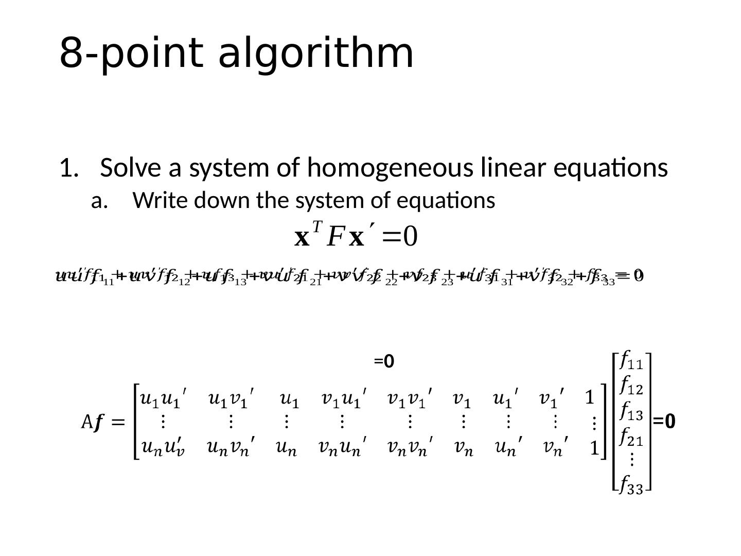
24 .8-point algorithm Solve a system of homogeneous linear equations Write down the system of equations   = 0  

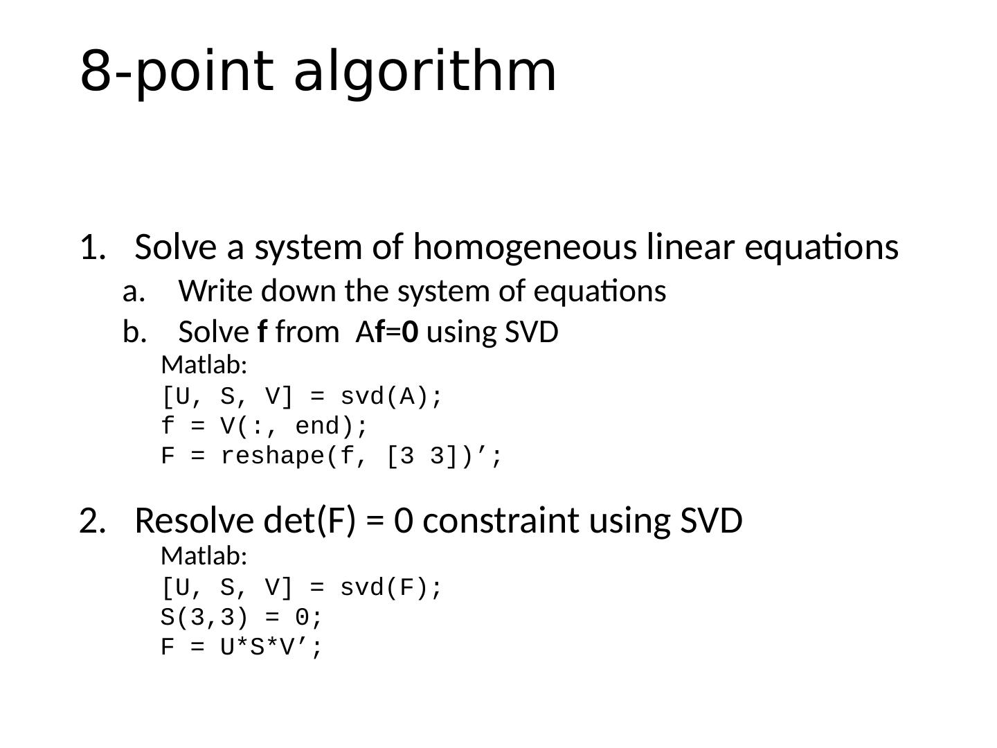
25 .8-point algorithm Solve a system of homogeneous linear equations Write down the system of equations Solve f from A f = 0 using SVD Matlab : [U, S, V] = svd (A); f = V(:, end); F = reshape(f, [3 3])’;

26 .Need to enforce singularity constraint

27 .8-point algorithm Solve a system of homogeneous linear equations Write down the system of equations Solve f from A f = 0 using SVD Resolve det (F) = 0 constraint using SVD Matlab : [U, S, V] = svd (A); f = V(:, end); F = reshape(f, [3 3])’; Matlab : [U, S, V] = svd (F); S(3,3) = 0; F = U*S*V’;

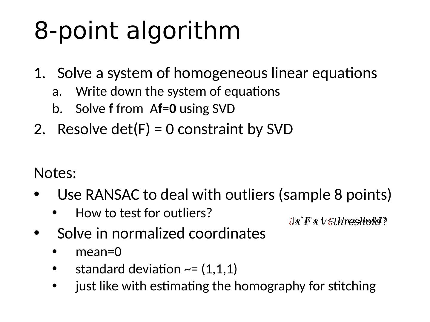
28 .8-point algorithm Solve a system of homogeneous linear equations Write down the system of equations Solve f from A f = 0 using SVD Resolve det (F) = 0 constraint by SVD Notes: Use RANSAC to deal with outliers (sample 8 points) How to test for outliers? Solve in normalized coordinates mean=0 s tandard deviation ~= (1,1,1) just like with estimating the homography for stitching  

29 .Homography (No Translation) Fundamental Matrix (Translation) Correspondence Relation Normalize image coordinates RANSAC with 8 points Initial solution via SVD Enforce by SVD De-normalize: Correspondence Relation Normalize image coordinates RANSAC with 4 points Solution via SVD De-normalize: Comparison of homography estimation and the 8-point algorithm Assume we have matched points x x ’ with outliers