基于运动视觉的稠密估计

1 .第八章 基于运动视觉的稠密估计 -------- 光流法 (OpticalOptical Flow)) 

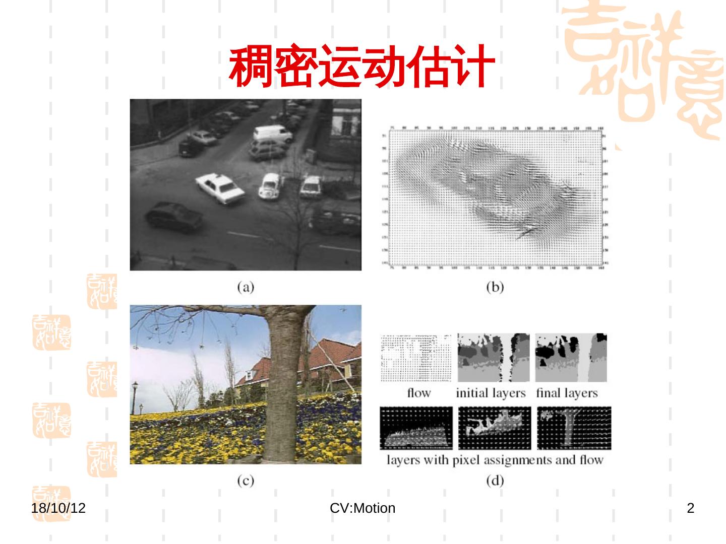
2 . 稠密运动估计 18/10/12 CV:Motion 2 

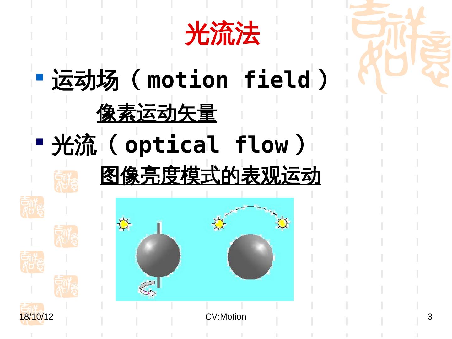
3 . 光流法  运动场（ motion field ） 像素运动矢量  光流（ optical flow ） 图像亮度模式的表观运动 18/10/12 CV:Motion 3 

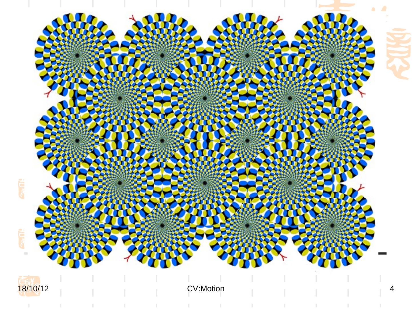
4 .18/10/12 CV:Motion 4 

5 . 8.1 二维光流运动估计  根据图像亮度模式的变化估计物体的运 动 1. 基于梯度的方法 (Gradient-Gradient- based) Differential Methods 2. 块匹配方法 (Gradient-Block Matching)) Reg)ion Matching) 18/10/12 CV:Motion 5 

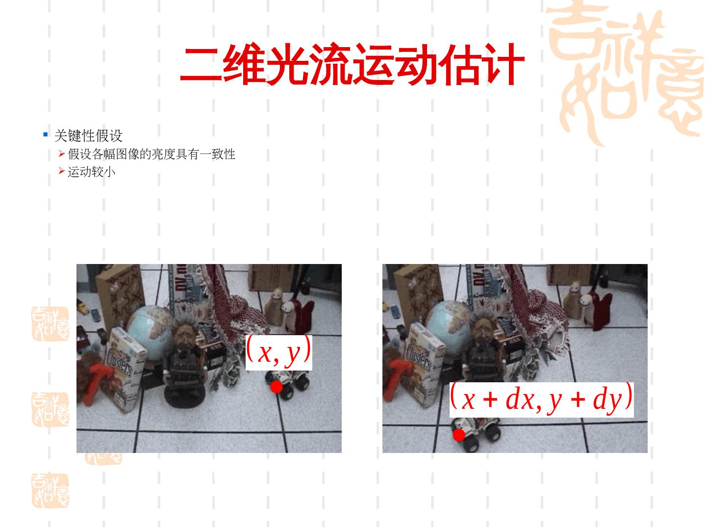
6 . 二维光流运动估计  关键性假设  假设各幅图像的亮度具有一致性  运动较小 Time = t Time = t+dt  x, y   x  dx , y  dy  I 0 ( x , y , t )  I1 ( x  x , y  y , t  t ) 

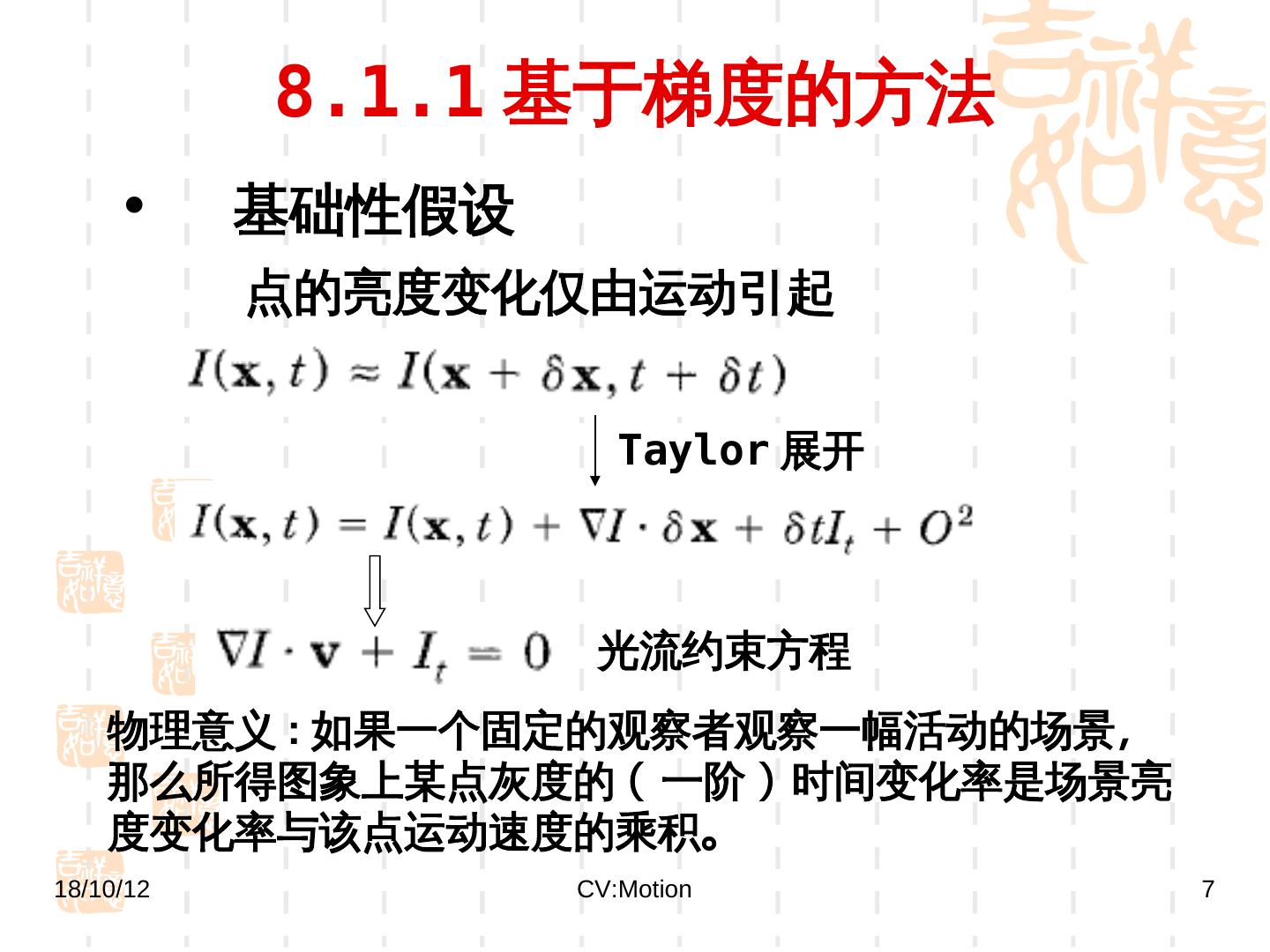
7 . 8.1.1 基于梯度的方法 • 基础性假设 点的亮度变化仅由运动引起 Taylor 展开 光流约束方程 物理意义 : 如果一个固定的观察者观察一幅活动的场景， 那么所得图象上某点灰度的 ( 一阶 ) 时间变化率是场景亮 度变化率与该点运动速度的乘积。 18/10/12 CV:Motion 7 

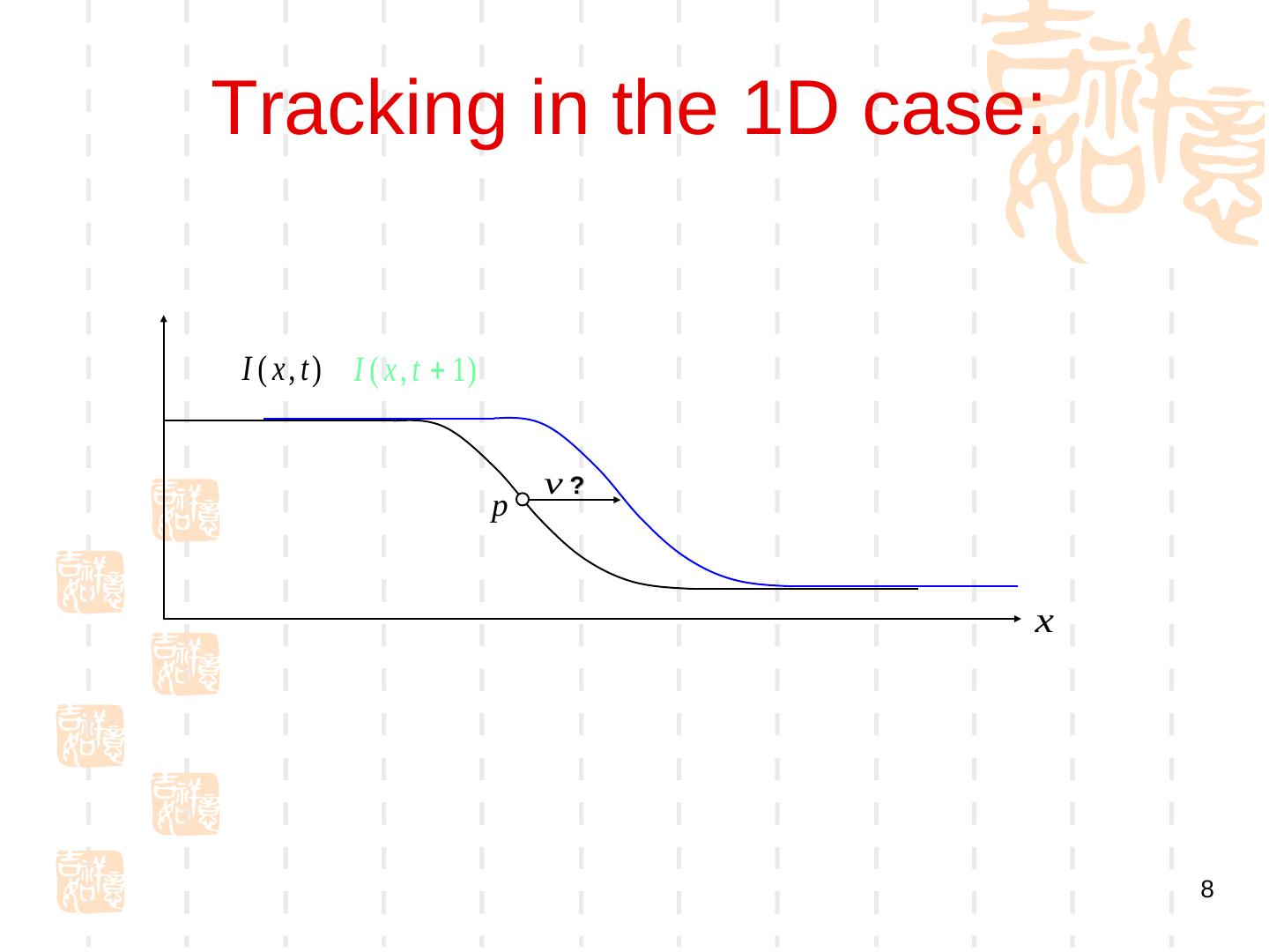
8 .Tracking in the 1D case: I ( x , t ) I ( x , t  1)  v? p x 8 

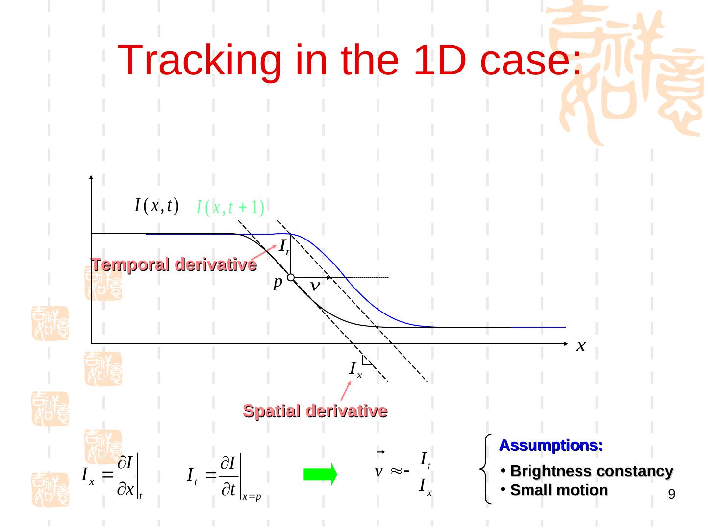
9 . Tracking in the 1D case: I ( x , t ) I ( x , t  1) It Temporal derivative p  v x Ix Spatial derivative Assumptions: I I  I Ix  It  v  t • Brightness constancy x t t x p Ix • Small motion 9 

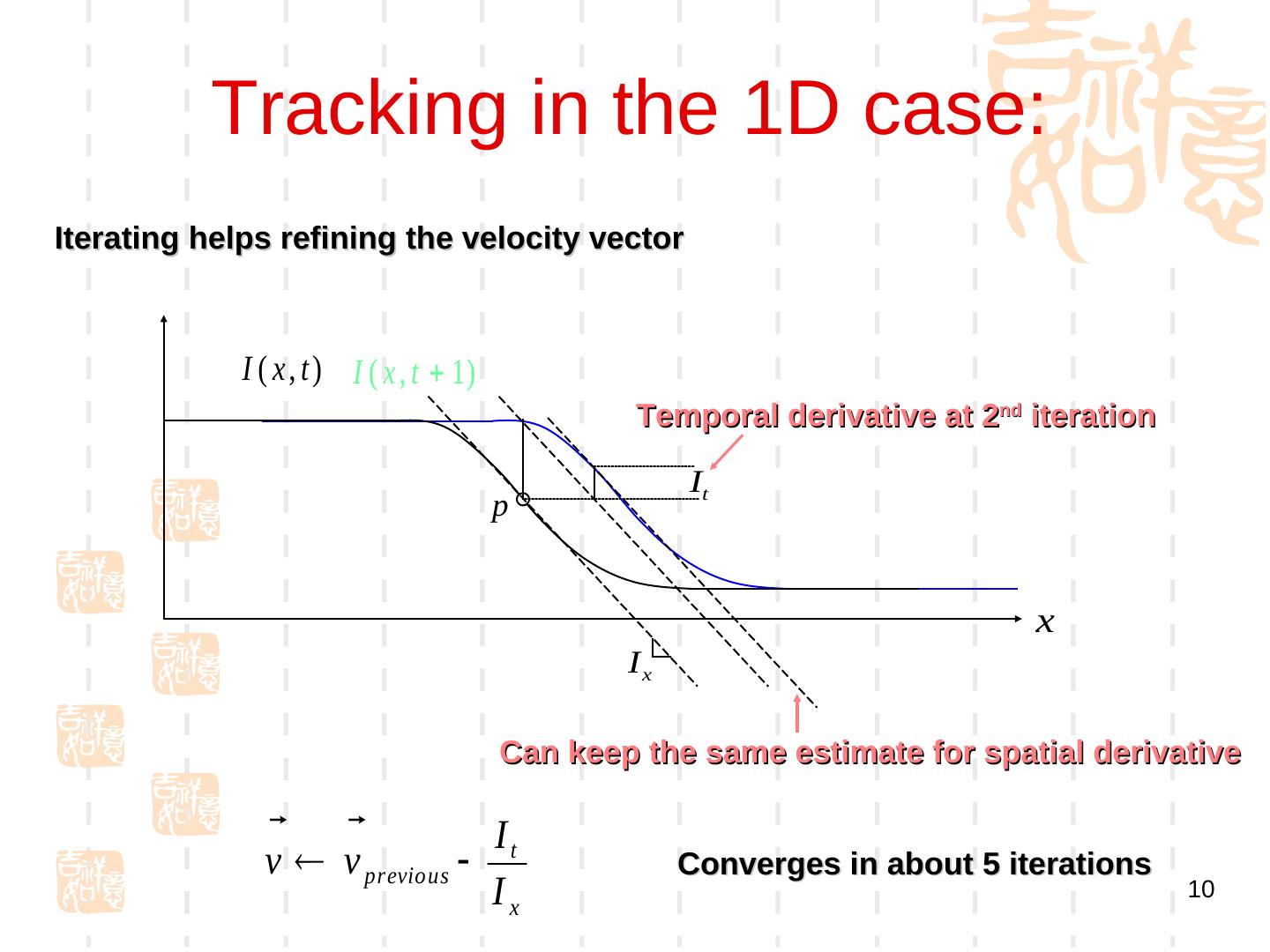
10 . Tracking in the 1D case: Iterating helps refining the velocity vector I ( x , t ) I ( x , t  1) Temporal derivative at 2nd iteration It p x Ix Can keep the same estimate for spatial derivative   I v  v previous  t Converges in about 5 iterations Ix 10 

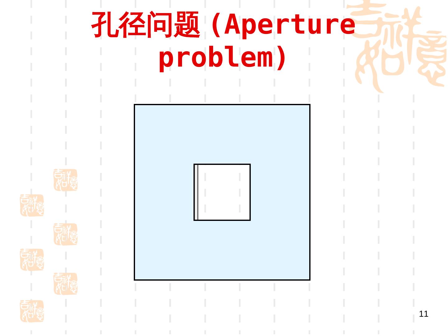
11 .孔径问题 (Gradient-Aperture problem) 11 

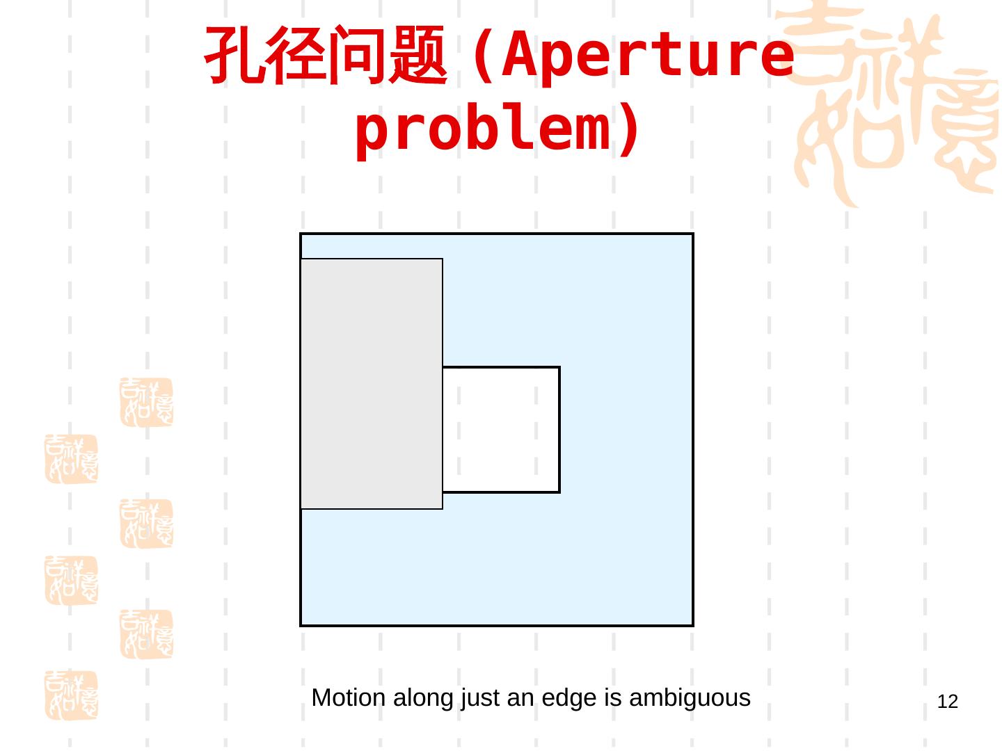
12 .孔径问题 (Gradient-Aperture problem) Motion along just an edge is ambiguous 12 

13 .孔径问题 (Gradient-Aperture problem) 13 

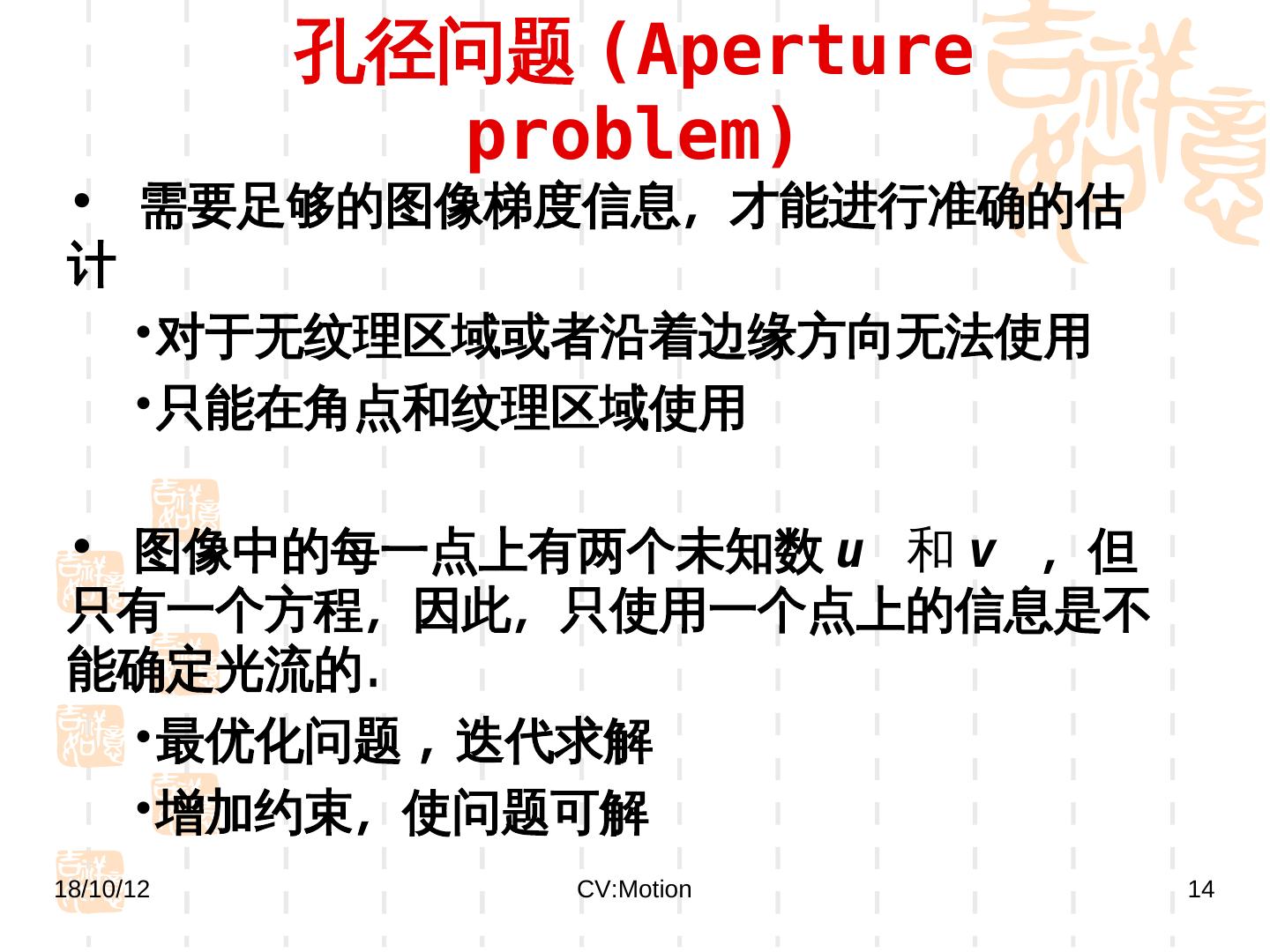
14 . 孔径问题 (Gradient-Aperture problem) • 需要足够的图像梯度信息，才能进行准确的估 计 •对于无纹理区域或者沿着边缘方向无法使用 •只能在角点和纹理区域使用 • 图像中的每一点上有两个未知数 u 和 v ，但 只有一个方程，因此，只使用一个点上的信息是不 能确定光流的． •最优化问题 , 迭代求解 •增加约束，使问题可解 18/10/12 CV:Motion 14 

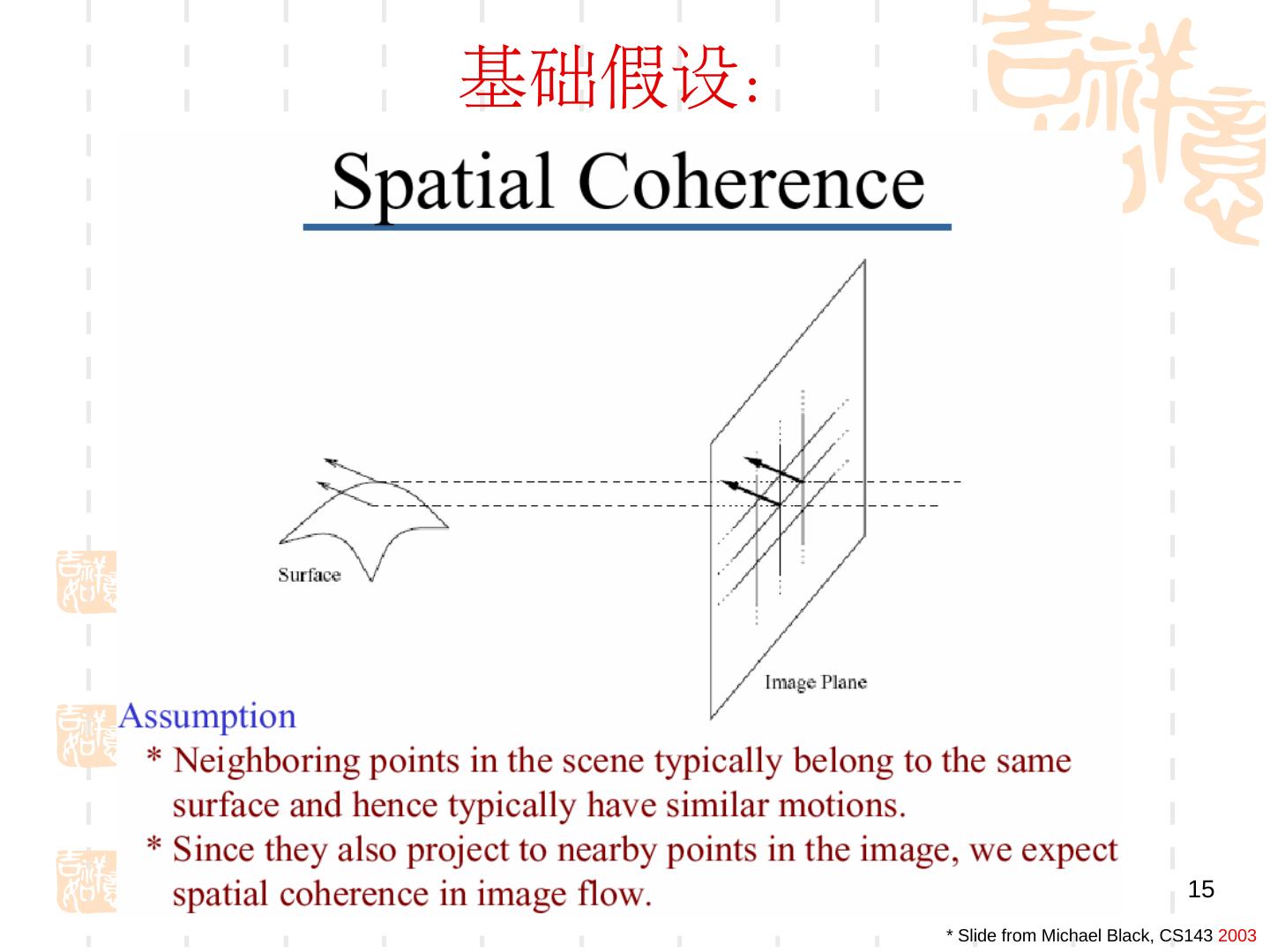
15 .基础假设： 15 * Slide from Michael Black, CS143 2003 

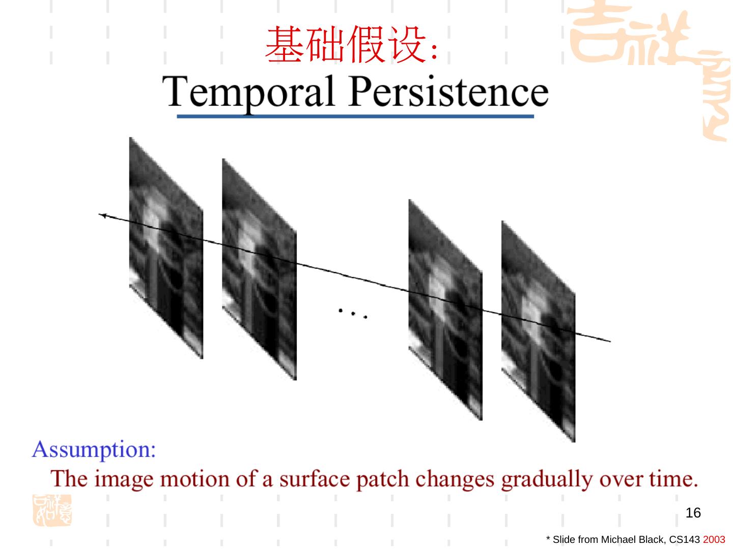
16 .基础假设： 16 * Slide from Michael Black, CS143 2003 

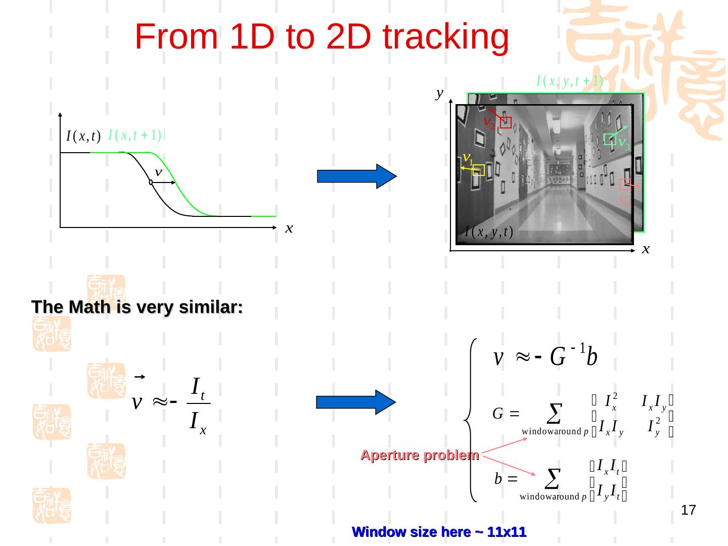
17 . From 1D to 2D tracking I ( x , y , t  1) y  v2 I ( x , t ) I ( x , t  1)   v3  v1 v  v4 x I ( x, y, t) x The Math is very similar:  v   G  1b  It v   I x2 IxIy Ix G   window around p  I x I y  I y2  Aperture problem  I x It  b    window around p  I y I t  17 Window) size here ~ 11x11 

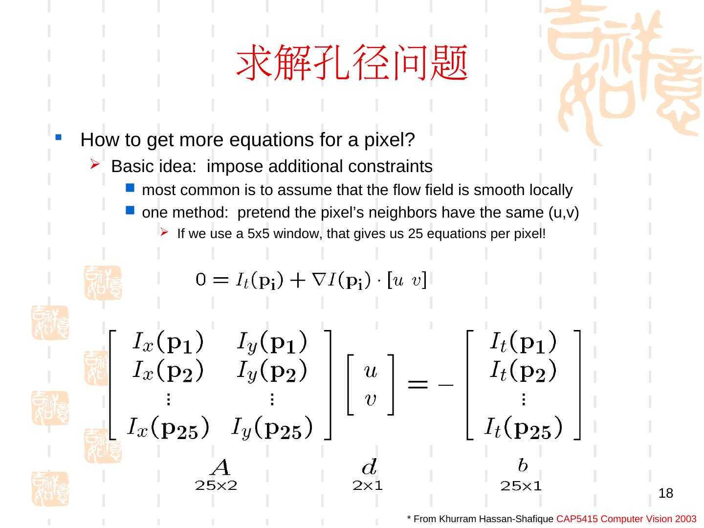
18 . 求解孔径问题  How to get more equations for a pixel?  Basic idea: impose additional constraints  most common is to assume that the flow field is smooth locally  one method: pretend the pixel’s neighbors have the same (u,v)  If we use a 5x5 window, that gives us 25 equations per pixel! 18 * From Khurram Hassan-Shafique CAP5415 Computer Vision 2003 

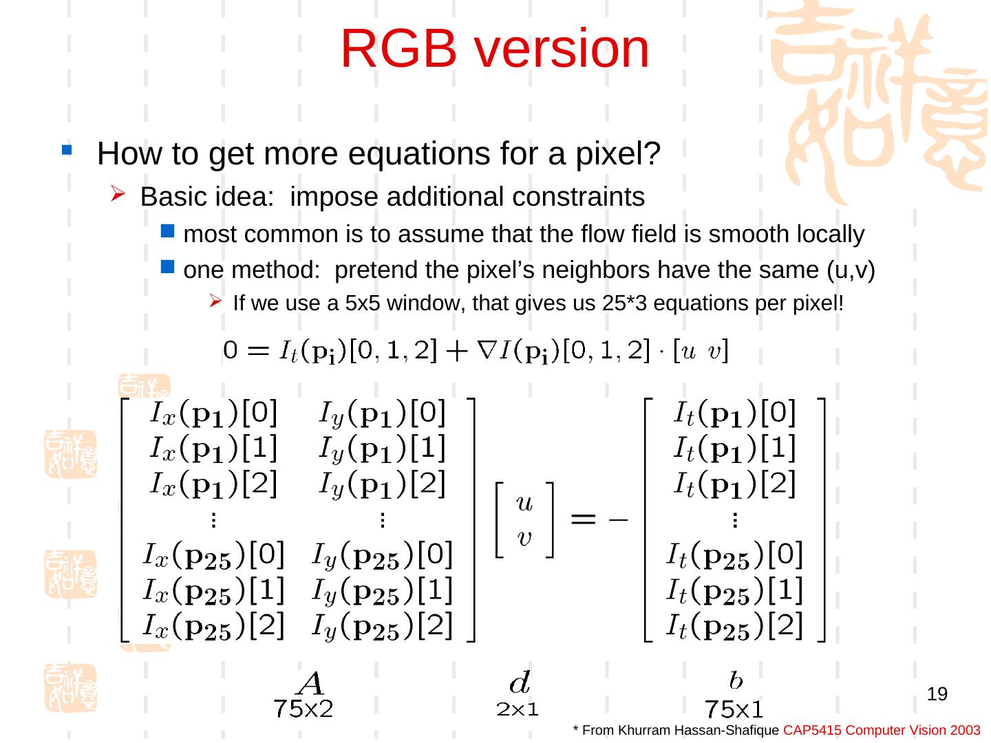
19 . RGB version  How to get more equations for a pixel?  Basic idea: impose additional constraints  most common is to assume that the flow field is smooth locally  one method: pretend the pixel’s neighbors have the same (u,v)  If we use a 5x5 window, that gives us 25*3 equations per pixel! 19 * From Khurram Hassan-Shafique CAP5415 Computer Vision 2003 

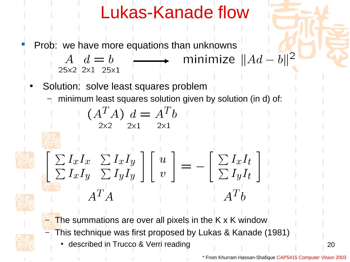
20 . Lukas-Kanade flow  Prob: we have more equations than unknowns • Solution: solve least squares problem – minimum least squares solution given by solution (in d) of: – The summations are over all pixels in the K x K window – This technique was first proposed by Lukas & Kanade (1981) • described in Trucco & Verri reading 20 * From Khurram Hassan-Shafique CAP5415 Computer Vision 2003 

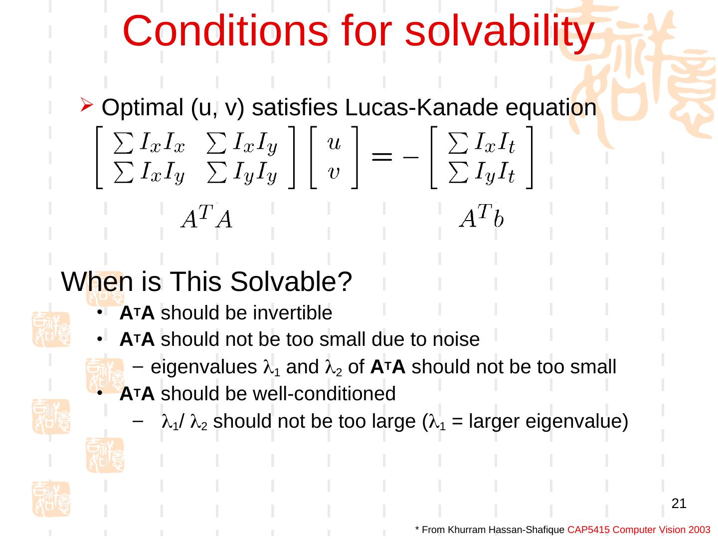
21 . Conditions for solvability  Optimal (u, v) satisfies Lucas-Kanade equation When is This Solvable? • ATA should be invertible • ATA should not be too small due to noise – eigenvalues 1 and 2 of ATA should not be too small • ATA should be well-conditioned – 1/ 2 should not be too large (1 = larger eigenvalue) 21 * From Khurram Hassan-Shafique CAP5415 Computer Vision 2003 

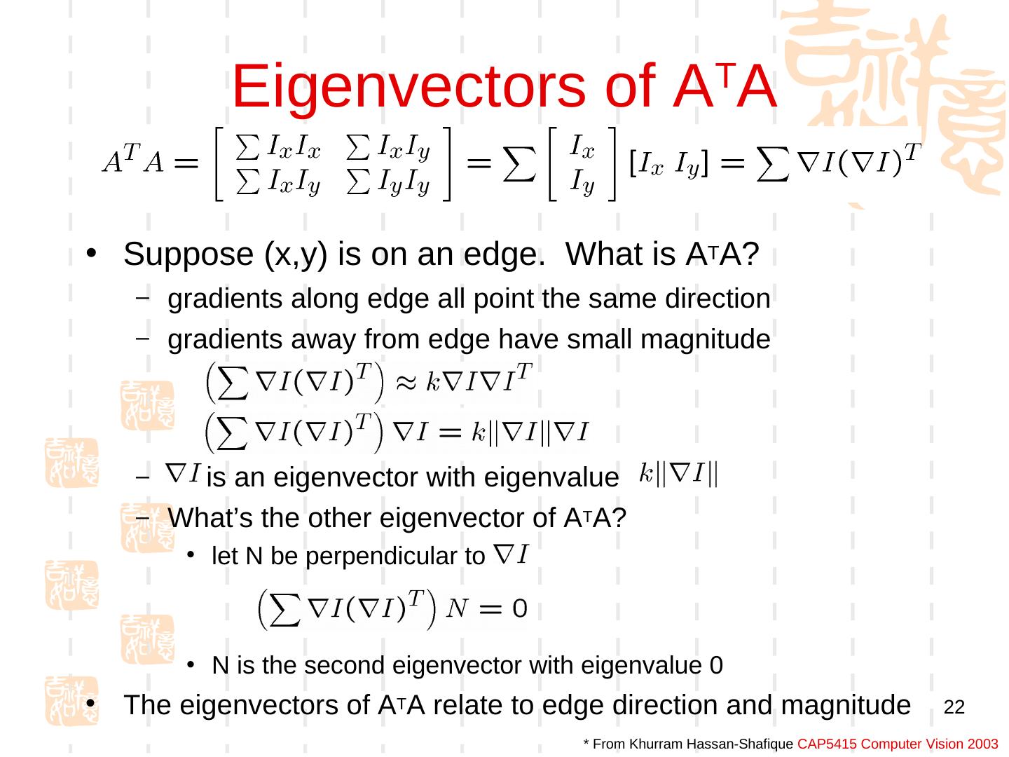
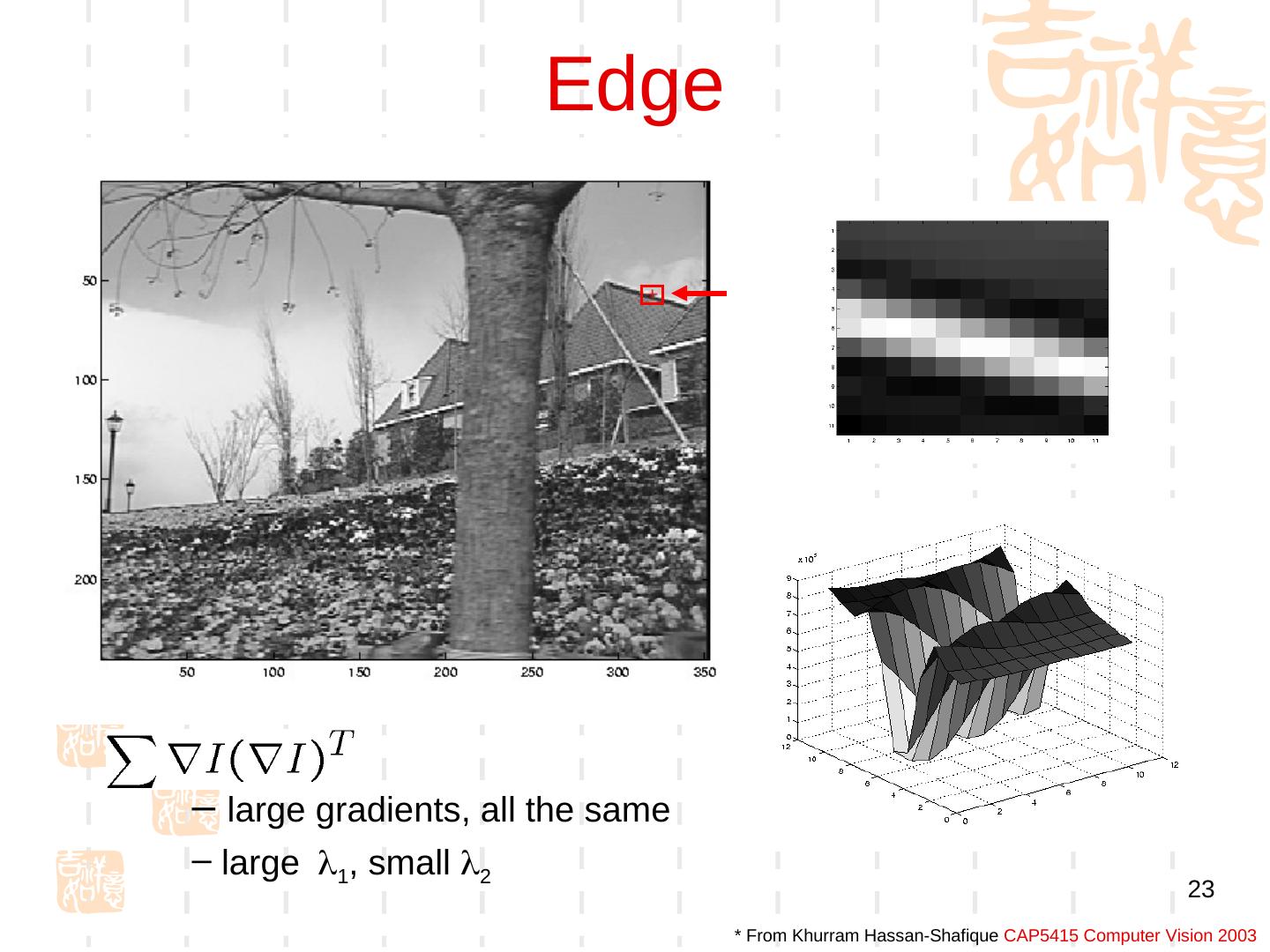
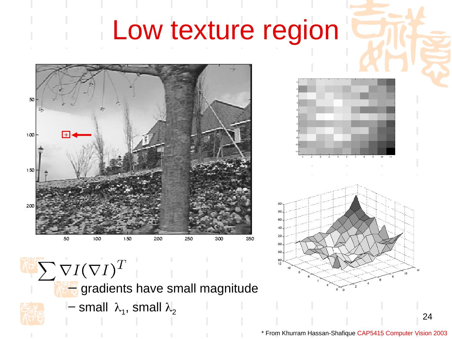
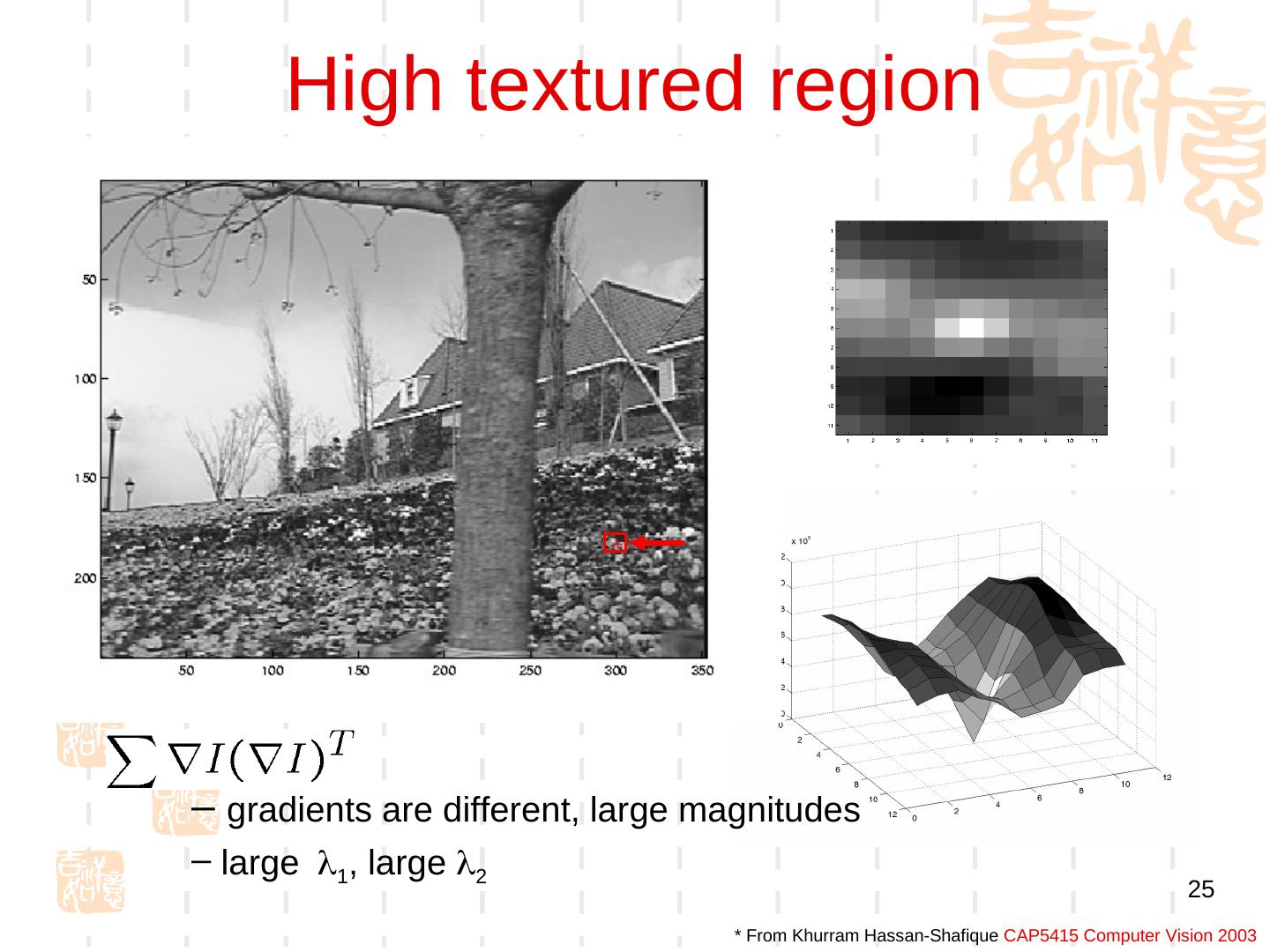
22 . Eigenvectors of A A T • Suppose (x,y) is on an edge. What is ATA? – gradients along edge all point the same direction – gradients away from edge have small magnitude – is an eigenvector with eigenvalue – What’s the other eigenvector of ATA? • let N be perpendicular to • N is the second eigenvector with eigenvalue 0 • The eigenvectors of ATA relate to edge direction and magnitude 22 * From Khurram Hassan-Shafique CAP5415 Computer Vision 2003 

23 . Edge – large gradients, all the same – large1, small 2 23 * From Khurram Hassan-Shafique CAP5415 Computer Vision 2003 

24 . Low texture region – gradients have small magnitude – small1, small 2 24 * From Khurram Hassan-Shafique CAP5415 Computer Vision 2003 

25 . High textured region – gradients are different, large magnitudes – large1, large 2 25 * From Khurram Hassan-Shafique CAP5415 Computer Vision 2003 

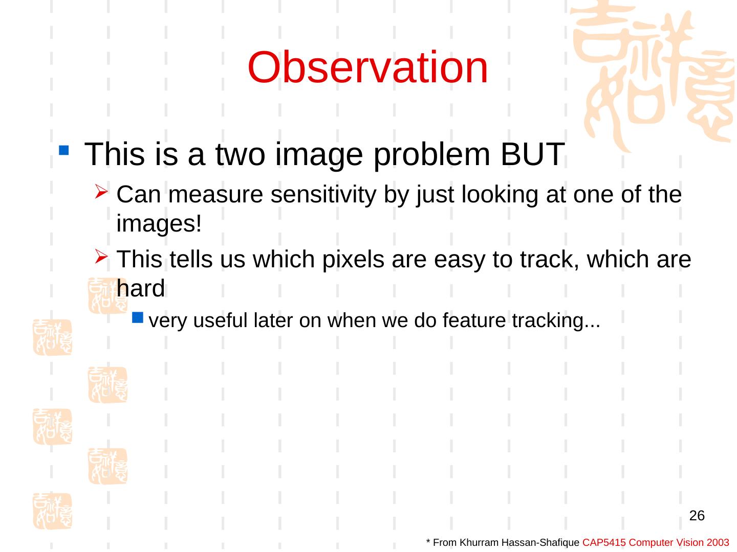
26 . Observation  This is a two image problem BUT  Can measure sensitivity by just looking at one of the images!  This tells us which pixels are easy to track, which are hard  very useful later on when we do feature tracking... 26 * From Khurram Hassan-Shafique CAP5415 Computer Vision 2003 

27 . 误差分析 What are the potential causes of errors in this procedure?  Suppose ATA is easily invertible  Suppose there is not much noise in the image • When our assumptions are violated – Brightness constancy is not satisfied – The motion is not small – A point does not move like its neighbors • window size is too large • what is the ideal window size? 27 * From Khurram Hassan-Shafique CAP5415 Computer Vision 2003 

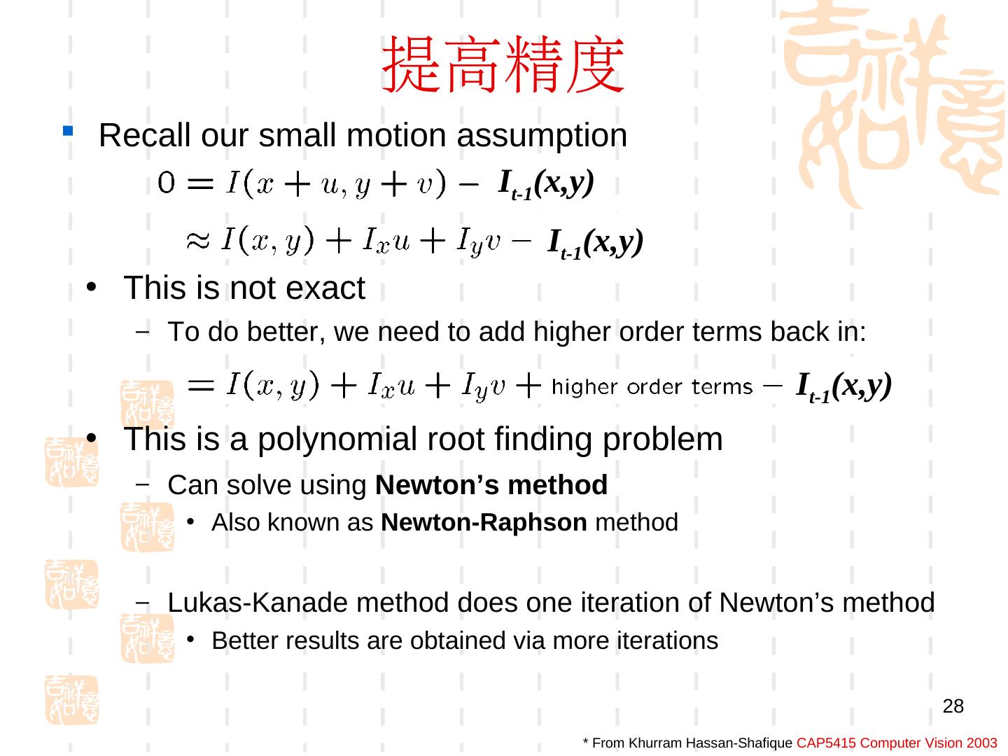
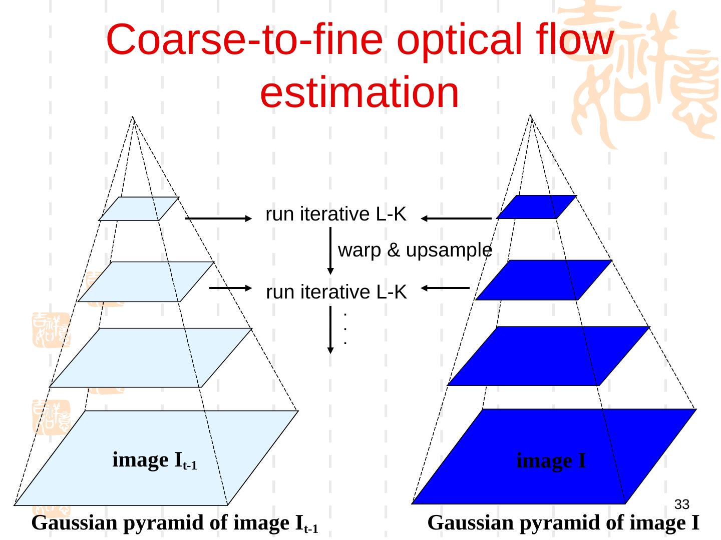
28 . 提高精度  Recall our small motion assumption It-1(x,y) It-1(x,y) • This is not exact – To do better, we need to add higher order terms back in: It-1(x,y) • This is a polynomial root finding problem – Can solve using New)ton’s method • Also known as New)ton-Raphson method – Lukas-Kanade method does one iteration of Newton’s method • Better results are obtained via more iterations 28 * From Khurram Hassan-Shafique CAP5415 Computer Vision 2003 

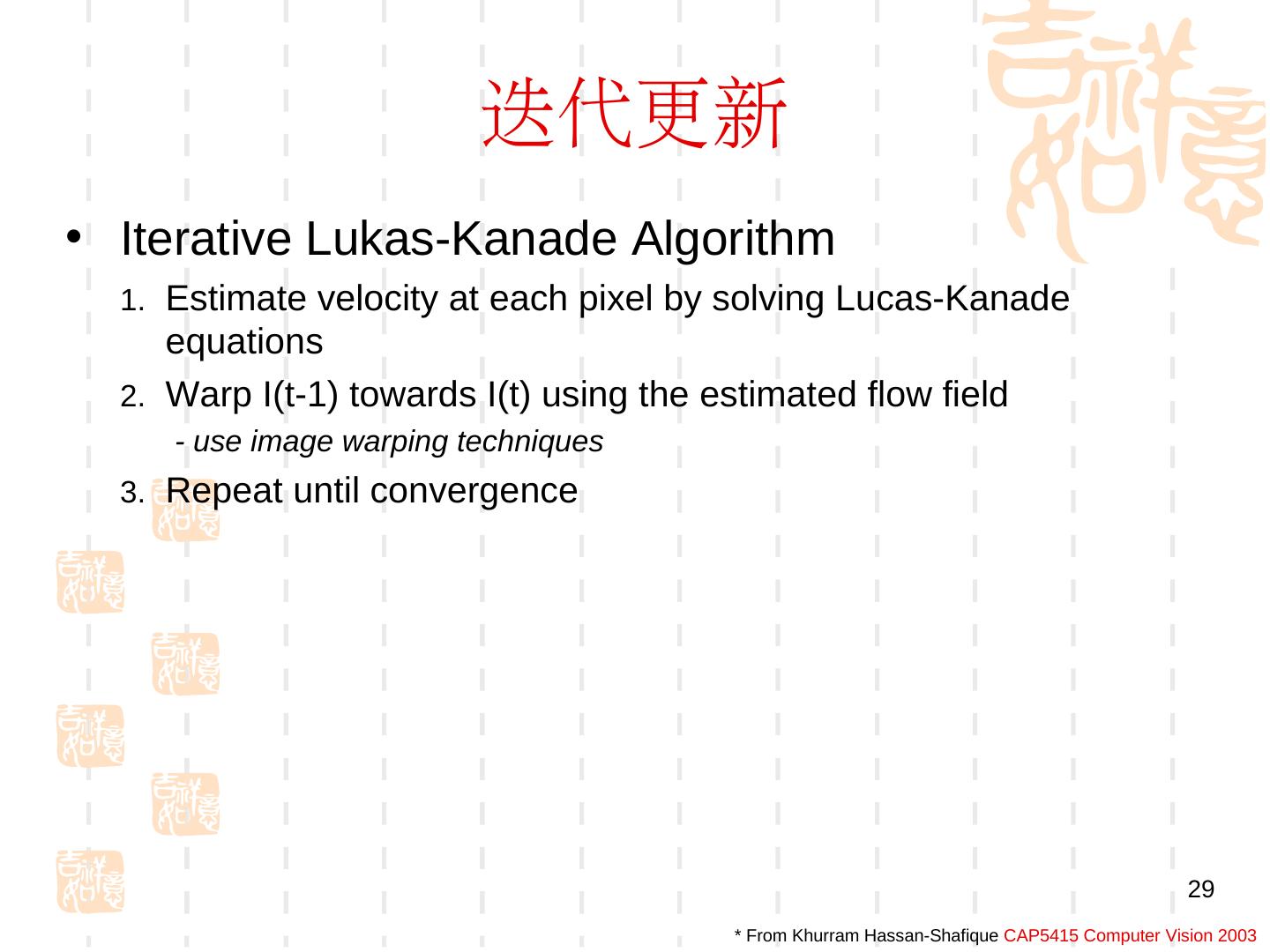
29 . 迭代更新 • Iterative Lukas-Kanade Algorithm 1. Estimate velocity at each pixel by solving Lucas-Kanade equations 2. Warp I(t-1) towards I(t) using the estimated flow field - use image warping techniques 3. Repeat until convergence 29 * From Khurram Hassan-Shafique CAP5415 Computer Vision 2003