分类; 聚类I

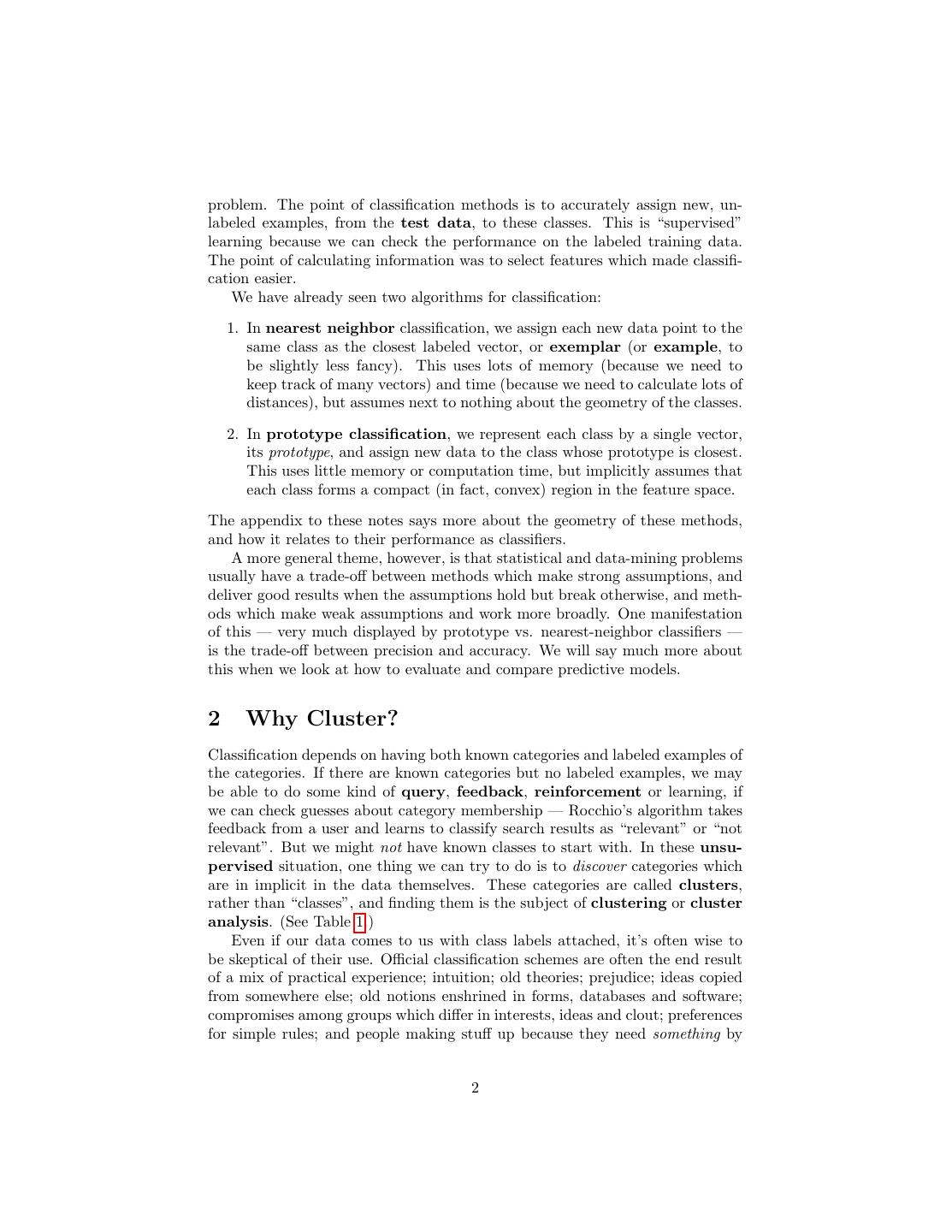
1 . Categorizing Data Vectors Types of Categorization, Basic Classifiers, Finding Simple Clusters in Data 36-350: Data Mining 11 September 2009 Reading: Textbook, sections 9.3–9.5. Contents 1 Categorization and Classifiers 1 2 Why Cluster? 2 2.1 Good clusters . . . . . . . . . . . . . . . . . . . . . . . . . . . . . 3 3 The k-means algorithm 4 3.1 Geometry of k-Means . . . . . . . . . . . . . . . . . . . . . . . . 5 3.2 k-Means as Search Algorithm . . . . . . . . . . . . . . . . . . . . 6 A Geometric Aspects of the Basic Classifiers 7 A.1 Prototype Method . . . . . . . . . . . . . . . . . . . . . . . . . . 7 A.1.1 Rate of Convergence . . . . . . . . . . . . . . . . . . . . . 8 A.2 Nearest-Neighbor Method . . . . . . . . . . . . . . . . . . . . . . 8 1 Categorization and Classifiers Dividing data into discrete categories is one of the most common kinds of data- mining task. Often the categories are things which are given to us in advance, by some kind of background knowledge (cells: cancerous or not?), or the kind of decision we are going to make (credit applicant: will they pay back the loan or not?), or simply by some taxonomy which our institution has decided to use (text: politics or religion? automobile or motorcycle?; pictures: flower, tiger or ocean?). This case, of assigning new data to pre-existing categories, is called classification, and the categories are called classes. When we have some examples, or training data, which have been labeled by someone who knew what they were doing, we have a supervised learning 1 

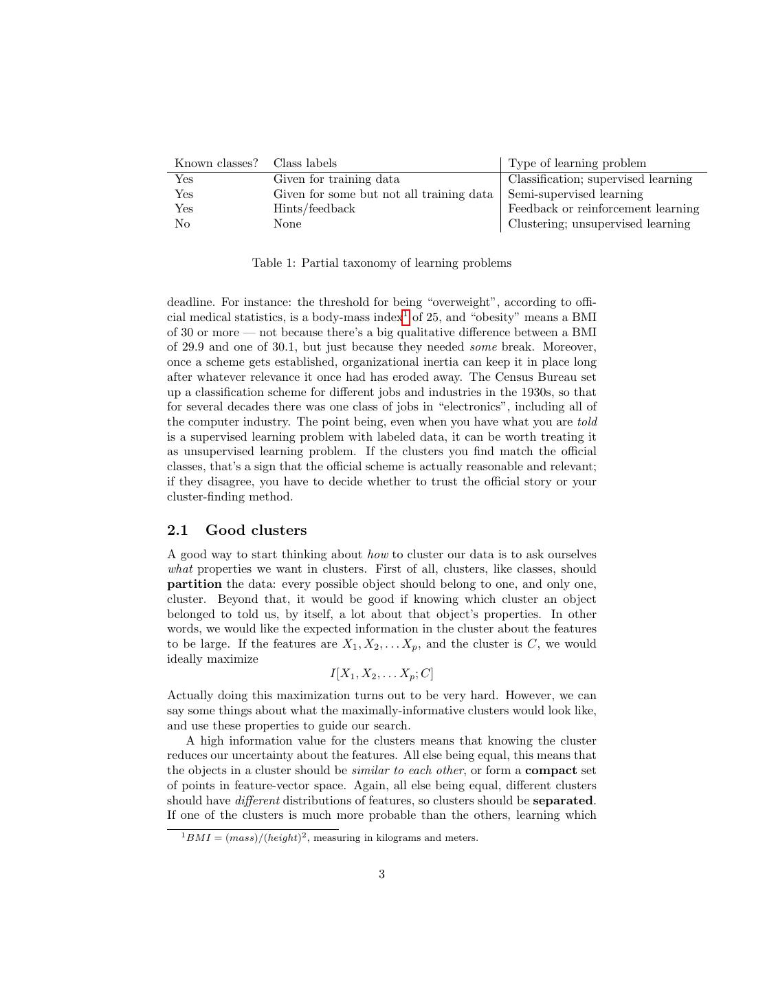
2 .problem. The point of classification methods is to accurately assign new, un- labeled examples, from the test data, to these classes. This is “supervised” learning because we can check the performance on the labeled training data. The point of calculating information was to select features which made classifi- cation easier. We have already seen two algorithms for classification: 1. In nearest neighbor classification, we assign each new data point to the same class as the closest labeled vector, or exemplar (or example, to be slightly less fancy). This uses lots of memory (because we need to keep track of many vectors) and time (because we need to calculate lots of distances), but assumes next to nothing about the geometry of the classes. 2. In prototype classification, we represent each class by a single vector, its prototype, and assign new data to the class whose prototype is closest. This uses little memory or computation time, but implicitly assumes that each class forms a compact (in fact, convex) region in the feature space. The appendix to these notes says more about the geometry of these methods, and how it relates to their performance as classifiers. A more general theme, however, is that statistical and data-mining problems usually have a trade-off between methods which make strong assumptions, and deliver good results when the assumptions hold but break otherwise, and meth- ods which make weak assumptions and work more broadly. One manifestation of this — very much displayed by prototype vs. nearest-neighbor classifiers — is the trade-off between precision and accuracy. We will say much more about this when we look at how to evaluate and compare predictive models. 2 Why Cluster? Classification depends on having both known categories and labeled examples of the categories. If there are known categories but no labeled examples, we may be able to do some kind of query, feedback, reinforcement or learning, if we can check guesses about category membership — Rocchio’s algorithm takes feedback from a user and learns to classify search results as “relevant” or “not relevant”. But we might not have known classes to start with. In these unsu- pervised situation, one thing we can try to do is to discover categories which are in implicit in the data themselves. These categories are called clusters, rather than “classes”, and finding them is the subject of clustering or cluster analysis. (See Table 1.) Even if our data comes to us with class labels attached, it’s often wise to be skeptical of their use. Official classification schemes are often the end result of a mix of practical experience; intuition; old theories; prejudice; ideas copied from somewhere else; old notions enshrined in forms, databases and software; compromises among groups which differ in interests, ideas and clout; preferences for simple rules; and people making stuff up because they need something by 2 

3 . Known classes? Class labels Type of learning problem Yes Given for training data Classification; supervised learning Yes Given for some but not all training data Semi-supervised learning Yes Hints/feedback Feedback or reinforcement learning No None Clustering; unsupervised learning Table 1: Partial taxonomy of learning problems deadline. For instance: the threshold for being “overweight”, according to offi- cial medical statistics, is a body-mass index1 of 25, and “obesity” means a BMI of 30 or more — not because there’s a big qualitative difference between a BMI of 29.9 and one of 30.1, but just because they needed some break. Moreover, once a scheme gets established, organizational inertia can keep it in place long after whatever relevance it once had has eroded away. The Census Bureau set up a classification scheme for different jobs and industries in the 1930s, so that for several decades there was one class of jobs in “electronics”, including all of the computer industry. The point being, even when you have what you are told is a supervised learning problem with labeled data, it can be worth treating it as unsupervised learning problem. If the clusters you find match the official classes, that’s a sign that the official scheme is actually reasonable and relevant; if they disagree, you have to decide whether to trust the official story or your cluster-finding method. 2.1 Good clusters A good way to start thinking about how to cluster our data is to ask ourselves what properties we want in clusters. First of all, clusters, like classes, should partition the data: every possible object should belong to one, and only one, cluster. Beyond that, it would be good if knowing which cluster an object belonged to told us, by itself, a lot about that object’s properties. In other words, we would like the expected information in the cluster about the features to be large. If the features are X1 , X2 , . . . Xp , and the cluster is C, we would ideally maximize I[X1 , X2 , . . . Xp ; C] Actually doing this maximization turns out to be very hard. However, we can say some things about what the maximally-informative clusters would look like, and use these properties to guide our search. A high information value for the clusters means that knowing the cluster reduces our uncertainty about the features. All else being equal, this means that the objects in a cluster should be similar to each other, or form a compact set of points in feature-vector space. Again, all else being equal, different clusters should have different distributions of features, so clusters should be separated. If one of the clusters is much more probable than the others, learning which 1 BM I = (mass)/(height)2 , measuring in kilograms and meters. 3 

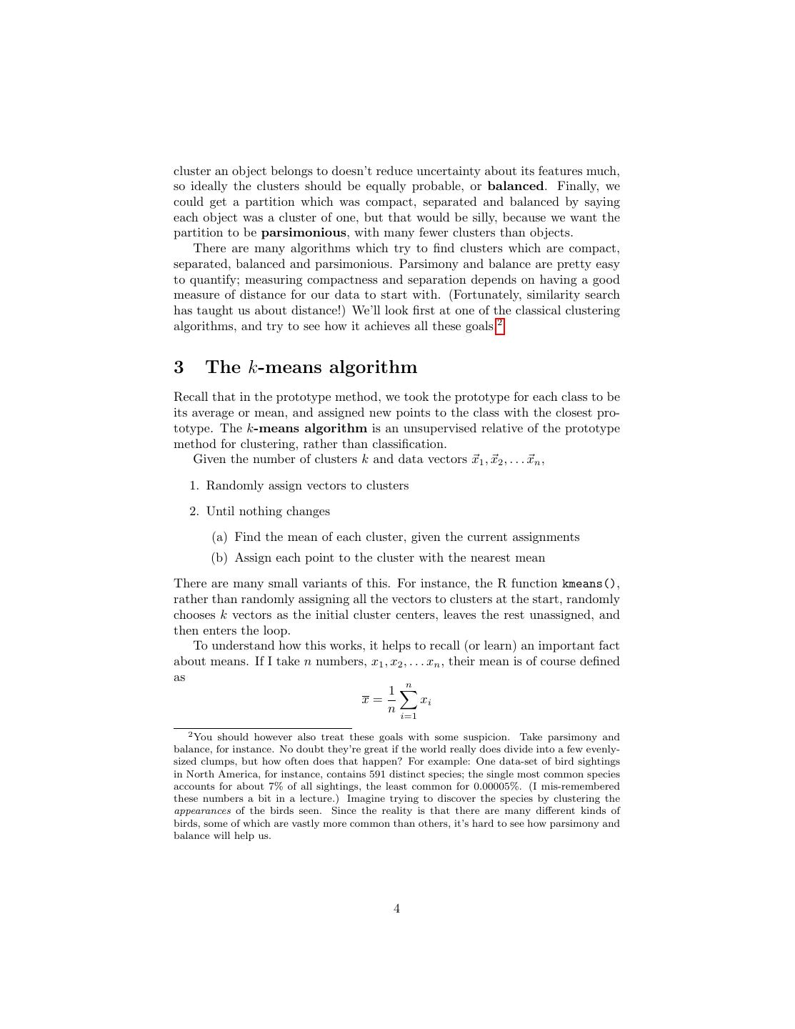
4 .cluster an object belongs to doesn’t reduce uncertainty about its features much, so ideally the clusters should be equally probable, or balanced. Finally, we could get a partition which was compact, separated and balanced by saying each object was a cluster of one, but that would be silly, because we want the partition to be parsimonious, with many fewer clusters than objects. There are many algorithms which try to find clusters which are compact, separated, balanced and parsimonious. Parsimony and balance are pretty easy to quantify; measuring compactness and separation depends on having a good measure of distance for our data to start with. (Fortunately, similarity search has taught us about distance!) We’ll look first at one of the classical clustering algorithms, and try to see how it achieves all these goals.2 3 The k-means algorithm Recall that in the prototype method, we took the prototype for each class to be its average or mean, and assigned new points to the class with the closest pro- totype. The k-means algorithm is an unsupervised relative of the prototype method for clustering, rather than classification. Given the number of clusters k and data vectors x1 , x2 , . . . xn , 1. Randomly assign vectors to clusters 2. Until nothing changes (a) Find the mean of each cluster, given the current assignments (b) Assign each point to the cluster with the nearest mean There are many small variants of this. For instance, the R function kmeans(), rather than randomly assigning all the vectors to clusters at the start, randomly chooses k vectors as the initial cluster centers, leaves the rest unassigned, and then enters the loop. To understand how this works, it helps to recall (or learn) an important fact about means. If I take n numbers, x1 , x2 , . . . xn , their mean is of course defined as n 1 x= xi n i=1 2 You should however also treat these goals with some suspicion. Take parsimony and balance, for instance. No doubt they’re great if the world really does divide into a few evenly- sized clumps, but how often does that happen? For example: One data-set of bird sightings in North America, for instance, contains 591 distinct species; the single most common species accounts for about 7% of all sightings, the least common for 0.00005%. (I mis-remembered these numbers a bit in a lecture.) Imagine trying to discover the species by clustering the appearances of the birds seen. Since the reality is that there are many different kinds of birds, some of which are vastly more common than others, it’s hard to see how parsimony and balance will help us. 4 

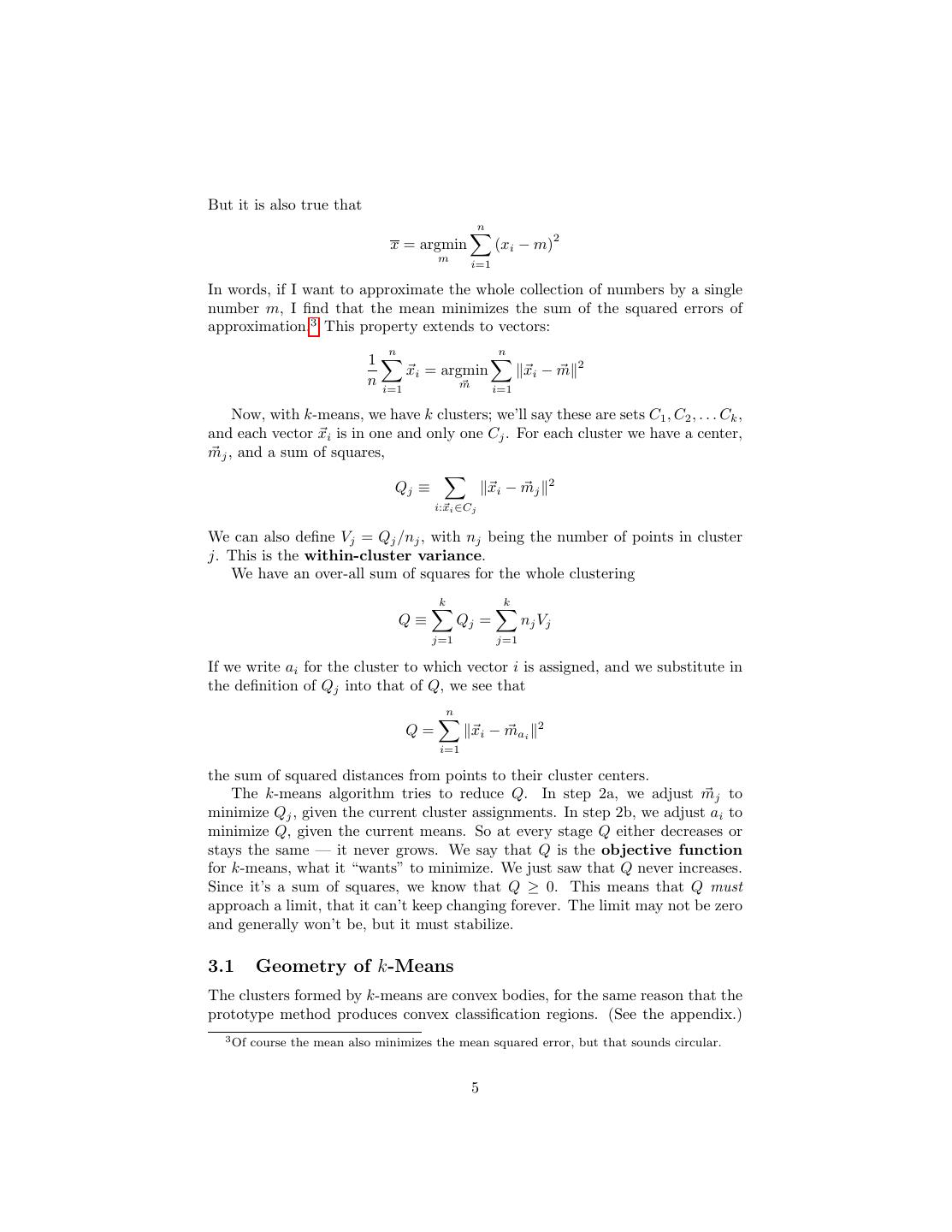
5 .But it is also true that n 2 x = argmin (xi − m) m i=1 In words, if I want to approximate the whole collection of numbers by a single number m, I find that the mean minimizes the sum of the squared errors of approximation.3 This property extends to vectors: n n 1 2 xi = argmin xi − m n i=1 m i=1 Now, with k-means, we have k clusters; we’ll say these are sets C1 , C2 , . . . Ck , and each vector xi is in one and only one Cj . For each cluster we have a center, mj , and a sum of squares, 2 Qj ≡ xi − mj i:xi ∈Cj We can also define Vj = Qj /nj , with nj being the number of points in cluster j. This is the within-cluster variance. We have an over-all sum of squares for the whole clustering k k Q≡ Qj = nj V j j=1 j=1 If we write ai for the cluster to which vector i is assigned, and we substitute in the definition of Qj into that of Q, we see that n 2 Q= xi − mai i=1 the sum of squared distances from points to their cluster centers. The k-means algorithm tries to reduce Q. In step 2a, we adjust mj to minimize Qj , given the current cluster assignments. In step 2b, we adjust ai to minimize Q, given the current means. So at every stage Q either decreases or stays the same — it never grows. We say that Q is the objective function for k-means, what it “wants” to minimize. We just saw that Q never increases. Since it’s a sum of squares, we know that Q ≥ 0. This means that Q must approach a limit, that it can’t keep changing forever. The limit may not be zero and generally won’t be, but it must stabilize. 3.1 Geometry of k-Means The clusters formed by k-means are convex bodies, for the same reason that the prototype method produces convex classification regions. (See the appendix.) 3 Of course the mean also minimizes the mean squared error, but that sounds circular. 5 

6 .This implies that if the true clusters aren’t convex regions of feature space, k-means cannot get them right. We can say a bit more about the geometry of the clusters. Remember that Q = j nj Vj , with nj being the number of points in the j th cluster, and Vj the within-cluster variance. If each cluster is compact, it will have a small within- cluster variance, so Vj and Q will be small, which k-means likes. Also, k-means tends to prefer equally-sized clusters, since all else being equal have n1 ≈ n2 makes n1 V1 +n2 V2 smaller. In other words, it favors balance, as discussed above. Finally, to minimize Vj around a given center, the points should be arranged in a circle (sphere, hyper-sphere) around that center, so the ideal cluster for k-means is a rounded blob. 3.2 k-Means as Search Algorithm K-means is a local search algorithm: it makes small changes to the solution that improve the objective. This sort of search strategy can get stuck in local minima, where the no improvement is possible by making small changes, but the objective function is still not optimized. It’s often helpful to think of this in terms of a search landscape, where the height of the landscape corresponds to how good a solution the algorithm has found. (So minimizing the objective function is the same as maximizing the height on the landscape.) Local search is also called hill climbing, because it’s like a short-sighted climber who tries to get to the top by always going uphill. If the landscape rises smoothly to a central peak, this will get to that peak. But if there are local peaks, it can get stuck at one, and which one it reaches depends on where the climb starts. For k-means, the different starting positions correspond to different initial guesses about the cluster centers. Changing those initial guesses will change the output of the algorithm. These are typically randomized, either as k random data points, or by randomly assigning points to clusters and then computing the means. Different runs of k-means will thus generally give different clusters, but you can actually make use of this: if some points end up clustered together in many different runs, that’s a good sign that they really do belong together. Exercises To think through, not to turn in. 1. Prove Eq. 3. (There are many ways to do this; the brute-force approach is to differentiate.) 2. Write your own k-means clustering algorithm. You may want to use the prototype classifier from the homework. 6 

7 .A Geometric Aspects of the Basic Classifiers This appendix goes over some of the geometry of the two basic classifier methods, and how this geometry connects to their statistical properties. A.1 Prototype Method Start with prototype classification. For each class i, i = 1, . . . k, we have a prototype vector ρi . We assign a new vector x to the class with the closest prototype: R(x) = argmin x − ρi (1) i In other words, R(x) = i if, and only if, x − ρi ≤ x − ρj , j = i. To see what this means, suppose that there are only two classes (i.e., k = 2). Then 1 x − ρ1 ≤ x − ρ2 R(x) = 2 x − ρ1 > x − ρ2 (This arbitrarily breaks the tie exactly on the boundary in favor of class 1. How we break the tie is immaterial.) What that means, as I drew on the board, is that the prototype method, in effect, draws the line segment from ρ1 to ρ2 , and then draws the perpendicular bisector of that line. (In d dimensions, the “perpendicular bisector” is a (d − 1)-dimensional hyperplane.) Everything on one side of the bisector goes into class 1, and everything on the other side goes into class 2. This divides the space into two half-spaces. Each half-space is a convex set, meaning that if x and y are both in the set, every point on the line-segment connecting them is also in the set. Now suppose there are more than two classes. The vector x gets assigned to class i if, and only if, it would be assigned to class i in every two-way match-up against the other classes. This means that the set of points which are assigned to the class i is the intersection of all of those half-spaces. Each half-space is a convex set, and the intersection of any number of convex sets is another convex set4 Thus, the prototype method represents the classes by convex sets (in fact by convex polygons, or their generalizations to higher dimensions). This will work well if the classes can, in fact, be well-approximated by convex sets. Examples like the bulls-eye pattern show situations where this implicit assumption of the prototype method fails spectacularly. The advantages of the prototype method are, once again, the limited amount of information to be stored (k prototype vectors), the fast computation to be performed (k distances calculations, and finding the smallest number from a list of k numbers), and the speed with which it converges to a final answer. 4A quibbler might ask, What if the two convex sets don’t overlap? Then their intersection is the empty set, which is technically convex. However, we know that ρi is closer to itself than is any other point, so all the half-spaces for class i have at least one point in common, and their intersection is therefore not empty. 7 

8 .A.1.1 Rate of Convergence Suppose that data vectors X1 , X2 , . . . are produced by independent and identically- distributed samples, and that the class Ci of a data-point depends determin- istically on the vector. That is, Ci = c(Xi ) for some function c(·). (We will see later how to handle the case where the feature vector doesn’t have enough information to perfectly classify cases.) For each class, then, there is a true mean vector: ρ∗i = E[X|c(X) = i] We don’t know the true means, but we can approximate them from our sample, and uses those approximations as our ρi : n k=1 Xk 1i Ck ρi = n k=1 1i Ck (This is just the mean of all the sample vectors whose class is i.) With IID samples, the law of large numbers tells us that ρi → ρ∗i . More than that, the central limit theorem tells us that |ρi − ρ∗i = O(n−1/2 ). Since the locations of the estimated centers determine the boundaries and so the classifi- cations, and the estimated centers converge rapidly, the classification function R(x) will converge rapidly to a limiting function.5 A.2 Nearest-Neighbor Method In the nearest-neighbor method, we have a set of data vectors x1 , x2 , . . . xn , each of which already has a class label, c1 , c2 , . . . cn . We then assign a new vector x to the class of its nearest neighbor: N (x) = argmin x − xi i C(x) = cN (x) Each of our example vectors xi thus has its own region of feature-space where it decides the class of new vectors. The analysis above for prototypes carries over: it’s the intersection of all the half-spaces which contain xi and divide it from the other points. So each xi gets its own convex set where it decides the class of new vectors. Since (in general) multiple examples have the same class label, each class corresponds to the union of several convex sets in feature space, and the union of convex sets is not (in general) convex. This gives nearest-neighbor classification more flexibility or expressive power than the prototype method. The price for the extra expressive power is paid in memory (in general, the algorithm needs to keep track of all the examples), in computational time (to calculate distances and find the shortest distance) and in the rate of convergence. 5 Unless some of the true class means are equal, i.e. ρ∗ = ρ∗ for some j = i. Then i and j i j will end up trying to divide the same cell of the partition, in an essentially random way that just reflects the difference in their sampling fluctuations. 8 

9 . With (as before) IID samples, the performance of the nearest neighbor rule is ultimately very good: if (as before) the class is a deterministic function of the features, Ci = c(Xi ), then in the long run the error rate of the nearest neighbor classifier goes to zero. More generally, if the class is only probabilistically related to the features, then the error rate converges to no more than twice the best attainable rate. Unfortunately the proof is a bit too complicated to go into here (Cover and Hart, 1967). As for the rate of convergence, the probability of error can shrink like 1/n2 , but it can also shrink arbitrarily slowly (Cover, 1968). References Cover, Thomas M. (1968). “Rates of Convergence for Nearest Neighbor Pro- cedures.” In Proceedings of the Hawaii International Conference on Systems Sciences (B. K. Kinariwala and F. F. Kuo, eds.), pp. 413–415. Honolulu: Uni- versity of Hawaii Press. URL http://www.stanford.edu/~cover/papers/ paper009.pdf. Cover, Thomas M. and P. E. Hart (1967). “Nearest Neighbor Pattern Clas- sification.” IEEE Transactions on Information Theory, 13: 21–27. URL http://www.stanford.edu/~cover/papers/transIT/0021cove.pdf. 9