- 快召唤伙伴们来围观吧
- 微博 QQ QQ空间 贴吧
- 文档嵌入链接
- <iframe src="https://www.slidestalk.com/u231/Dynamic_Programming?embed" frame border="0" width="640" height="360" scrolling="no" allowfullscreen="true">复制
- 微信扫一扫分享
动态规划
展开查看详情
1 . Dynamic Programming • A powerful paradigm for algorithm design. • Often leads to elegant and efficient algorithms when greedy or divide-and-conquer don’t work. • DP also breaks a problem into subproblems, but subproblems are not independent. • DP tabulates solutions of subproblems to avoid solving them again. Subhash Suri UC Santa Barbara
2 . Dynamic Programming • Typically applied to optimization problems: many feasible solutions; find one of optimal value. • Key is the principle of optimality: solution composed of optimal subproblem solutions. • Example: Matrix Chain Product. • A sequence M1, M2, . . . , Mn of n matrices to be multiplied. • Adjacent matrices must agree on dim. Subhash Suri UC Santa Barbara
3 . Matrix Product Matrix-Multiply (A, B) 1. Let A be p × q; let B be q × r. 2. If dim of A and B don’t agree, error. 3. for i = 1 to p 4. for j = 1 to r 5. C[i, j] = 0 6. for k = 1 to q 7. C[i, j] + = A[i, k] × B[k, j] 8. return C. • Cost of multiplying these matrices is p × q × r. Subhash Suri UC Santa Barbara
4 . Matrix Chain • Consider 4 matrices: M1, M2, M3, M4. • We can compute the product in many different ways, depending on how we parenthesize. (M1(M2(M3M4))) (M1((M2M3)M4)) ((M1M2)(M3M4)) (((M1M2)M3)M4) • Different multiplication orders can lead to very different total costs. Subhash Suri UC Santa Barbara
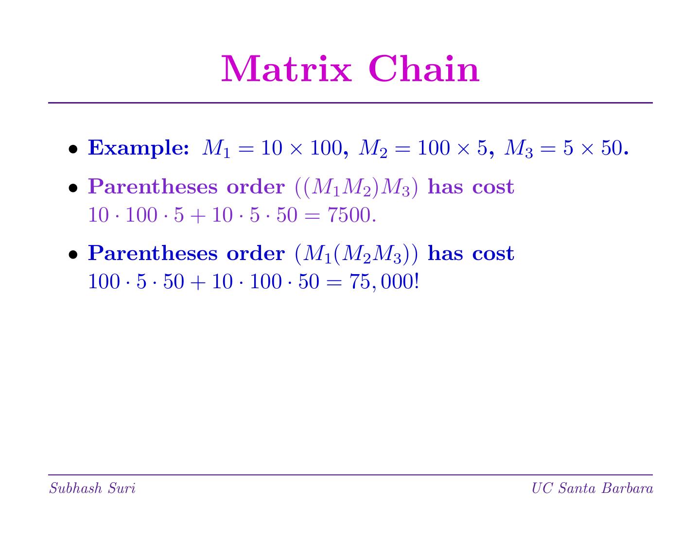
5 . Matrix Chain • Example: M1 = 10 × 100, M2 = 100 × 5, M3 = 5 × 50. • Parentheses order ((M1M2)M3) has cost 10 · 100 · 5 + 10 · 5 · 50 = 7500. • Parentheses order (M1(M2M3)) has cost 100 · 5 · 50 + 10 · 100 · 50 = 75, 000! Subhash Suri UC Santa Barbara
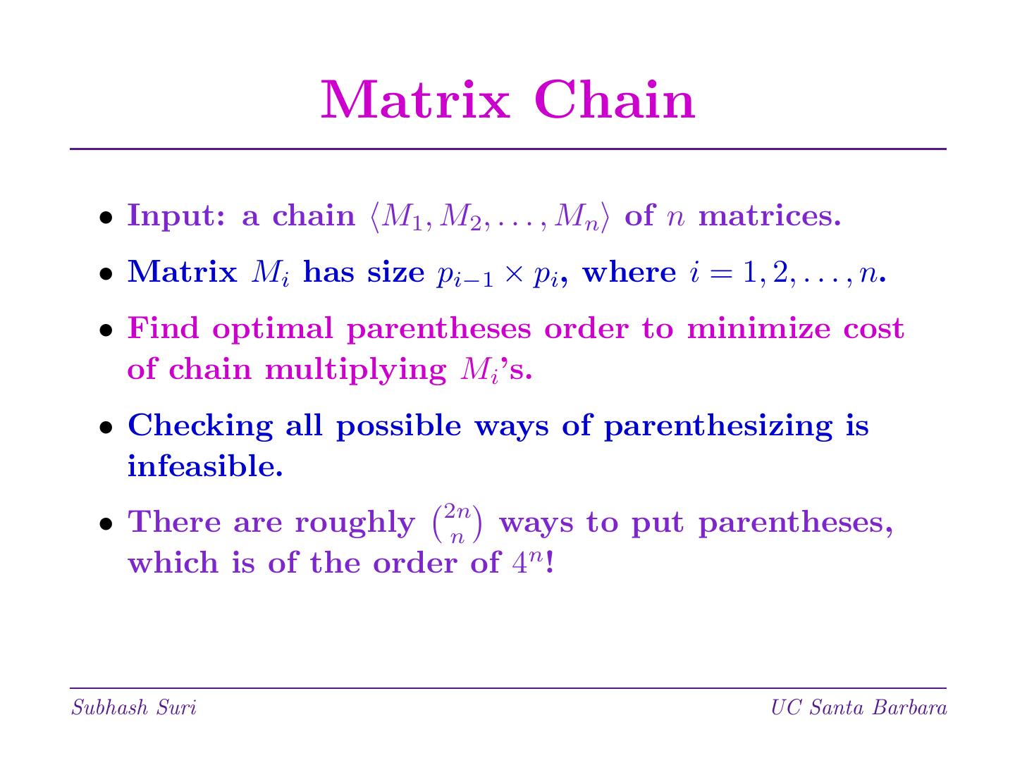
6 . Matrix Chain • Input: a chain M1, M2, . . . , Mn of n matrices. • Matrix Mi has size pi−1 × pi, where i = 1, 2, . . . , n. • Find optimal parentheses order to minimize cost of chain multiplying Mi’s. • Checking all possible ways of parenthesizing is infeasible. • There are roughly 2nn ways to put parentheses, which is of the order of 4n! Subhash Suri UC Santa Barbara
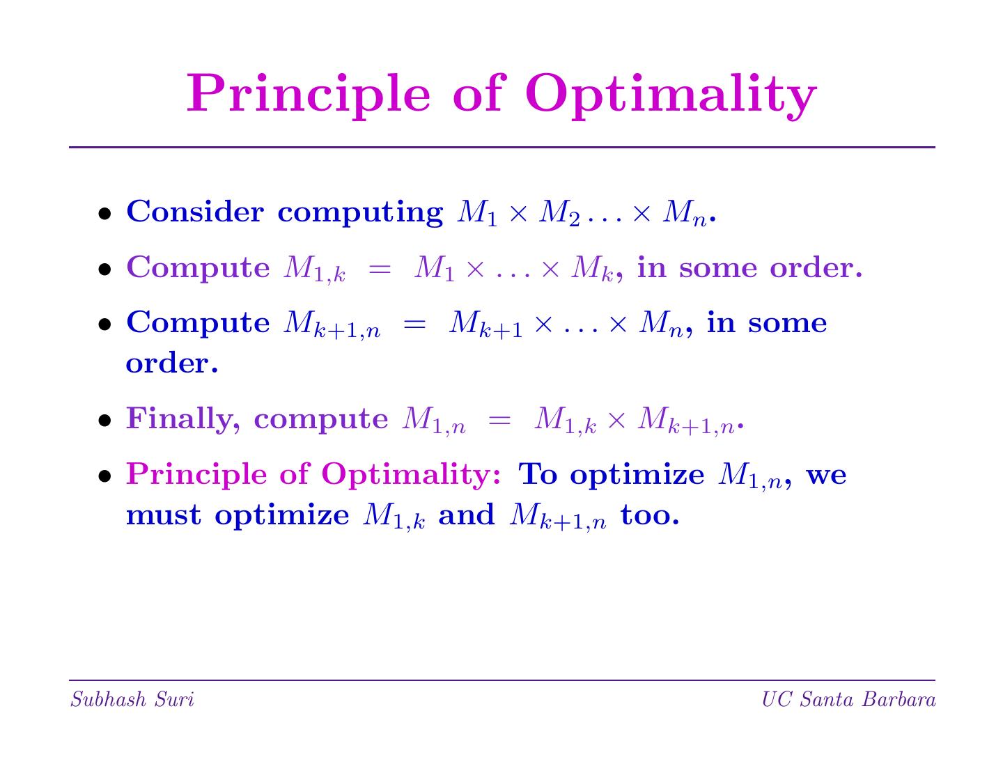
7 . Principle of Optimality • Consider computing M1 × M2 . . . × Mn. • Compute M1,k = M1 × . . . × Mk , in some order. • Compute Mk+1,n = Mk+1 × . . . × Mn, in some order. • Finally, compute M1,n = M1,k × Mk+1,n. • Principle of Optimality: To optimize M1,n, we must optimize M1,k and Mk+1,n too. Subhash Suri UC Santa Barbara
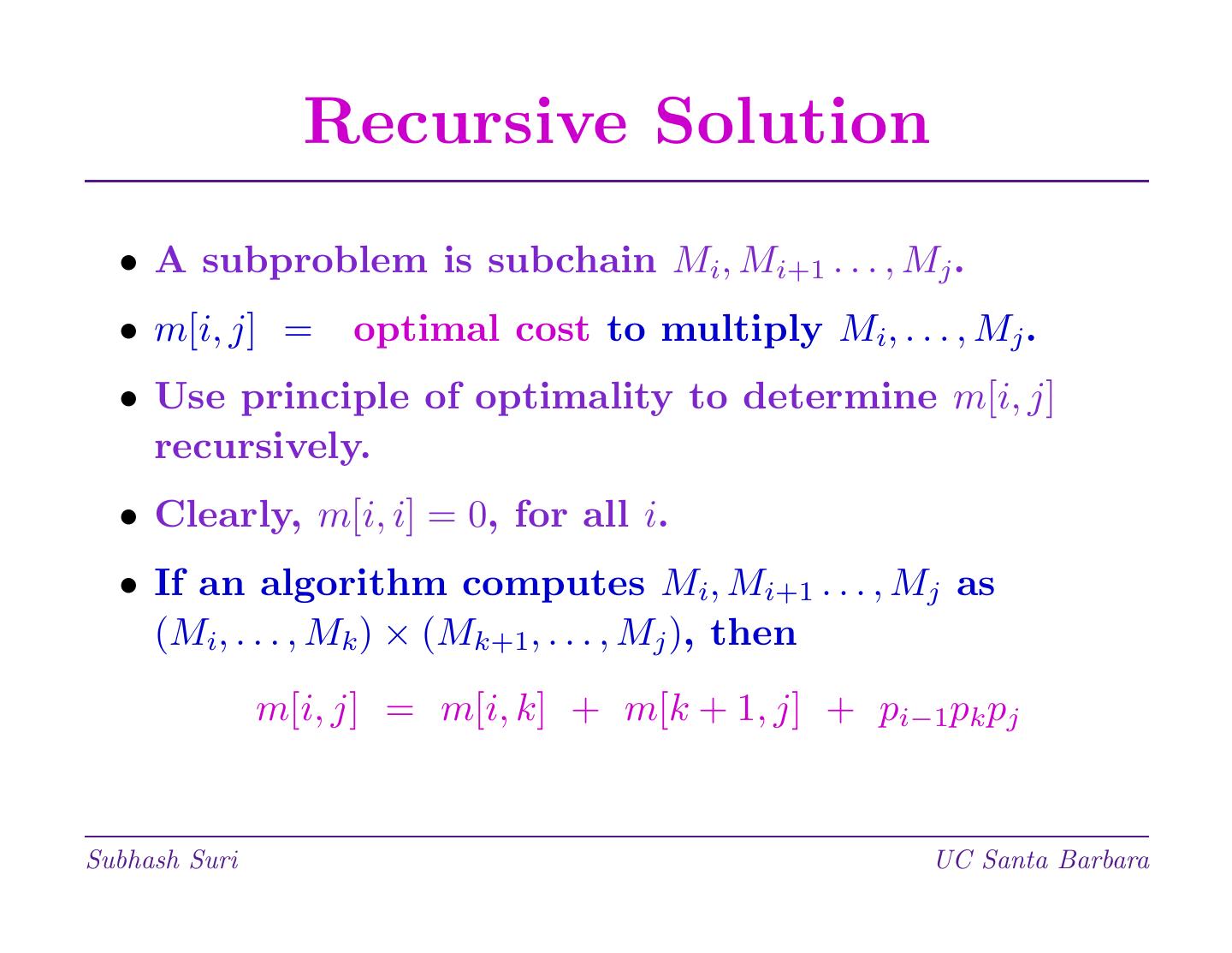
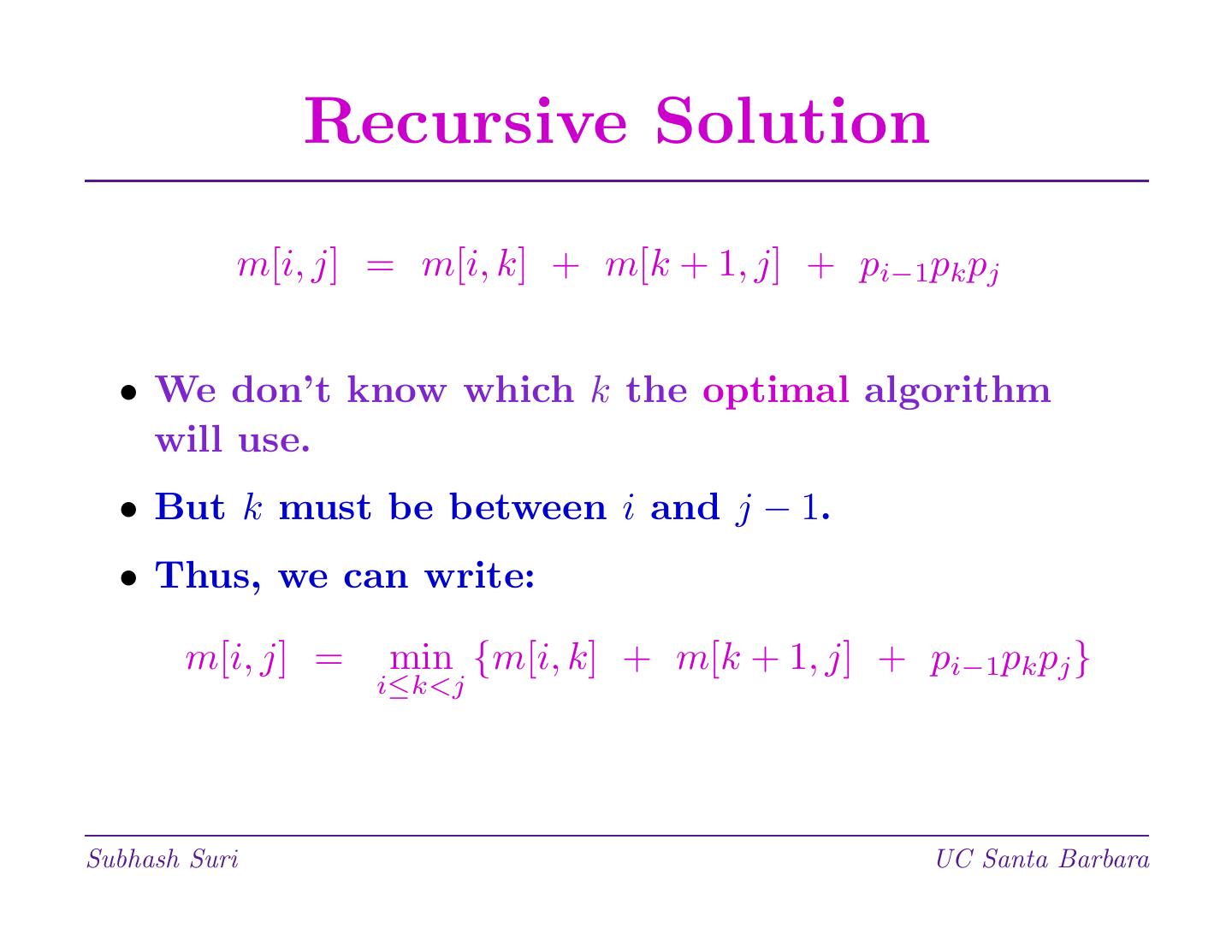
8 . Recursive Solution • A subproblem is subchain Mi, Mi+1 . . . , Mj . • m[i, j] = optimal cost to multiply Mi, . . . , Mj . • Use principle of optimality to determine m[i, j] recursively. • Clearly, m[i, i] = 0, for all i. • If an algorithm computes Mi, Mi+1 . . . , Mj as (Mi, . . . , Mk ) × (Mk+1, . . . , Mj ), then m[i, j] = m[i, k] + m[k + 1, j] + pi−1pk pj Subhash Suri UC Santa Barbara
9 . Recursive Solution m[i, j] = m[i, k] + m[k + 1, j] + pi−1pk pj • We don’t know which k the optimal algorithm will use. • But k must be between i and j − 1. • Thus, we can write: m[i, j] = min {m[i, k] + m[k + 1, j] + pi−1pk pj } i≤k<j Subhash Suri UC Santa Barbara
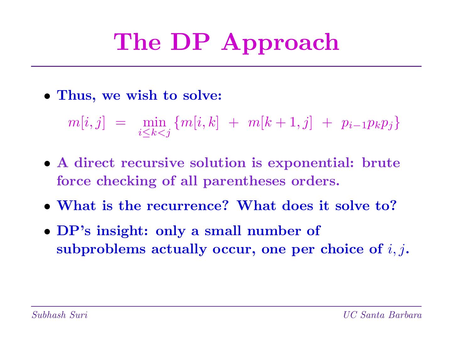
10 . The DP Approach • Thus, we wish to solve: m[i, j] = min {m[i, k] + m[k + 1, j] + pi−1pk pj } i≤k<j • A direct recursive solution is exponential: brute force checking of all parentheses orders. • What is the recurrence? What does it solve to? • DP’s insight: only a small number of subproblems actually occur, one per choice of i, j. Subhash Suri UC Santa Barbara
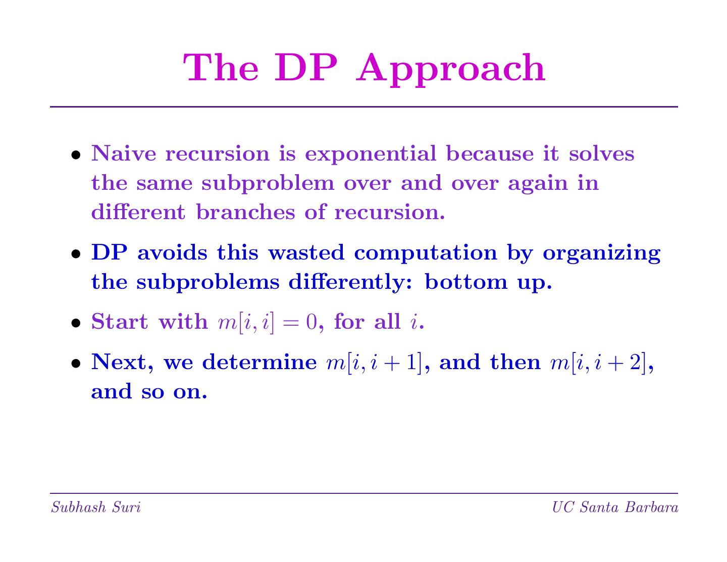
11 . The DP Approach • Naive recursion is exponential because it solves the same subproblem over and over again in different branches of recursion. • DP avoids this wasted computation by organizing the subproblems differently: bottom up. • Start with m[i, i] = 0, for all i. • Next, we determine m[i, i + 1], and then m[i, i + 2], and so on. Subhash Suri UC Santa Barbara
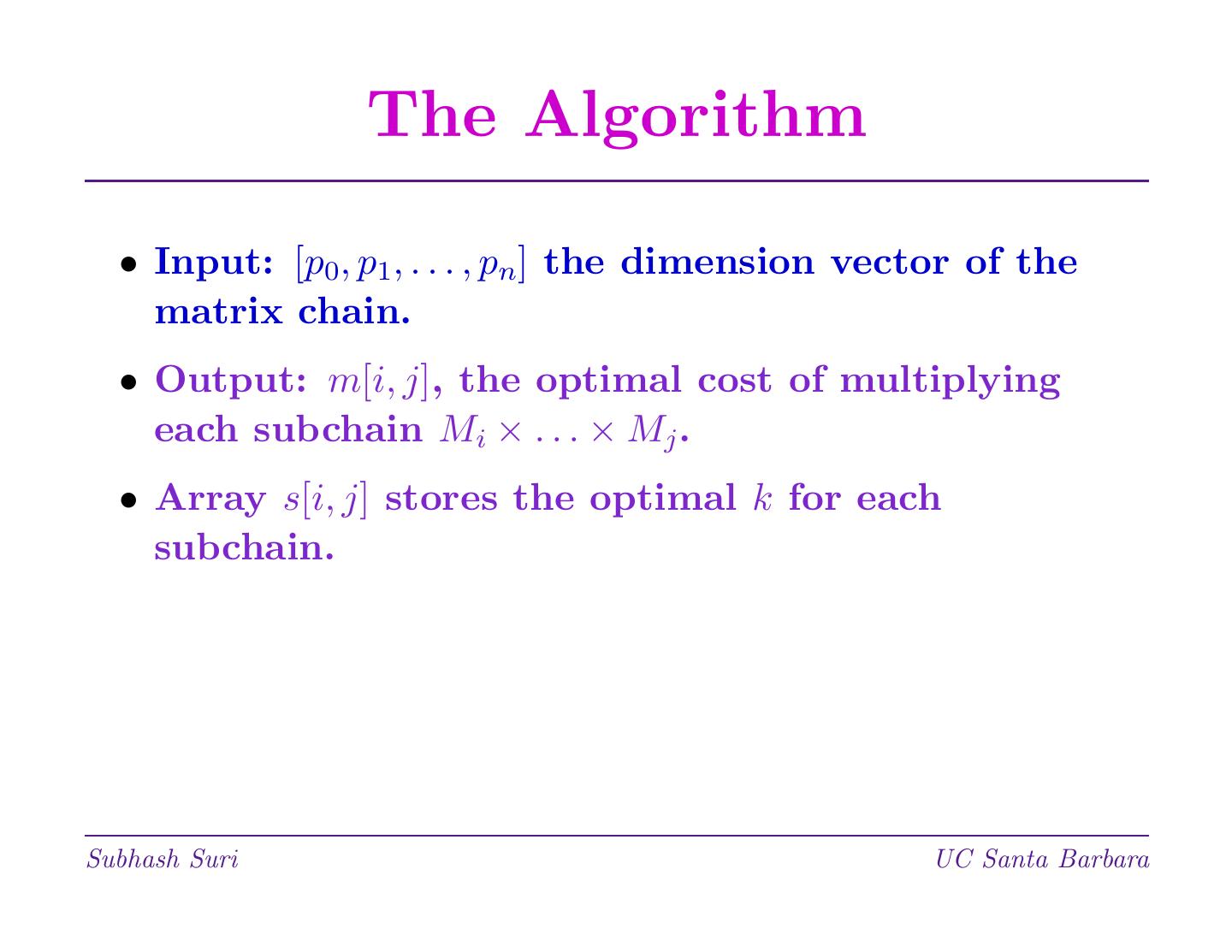
12 . The Algorithm • Input: [p0, p1, . . . , pn] the dimension vector of the matrix chain. • Output: m[i, j], the optimal cost of multiplying each subchain Mi × . . . × Mj . • Array s[i, j] stores the optimal k for each subchain. Subhash Suri UC Santa Barbara
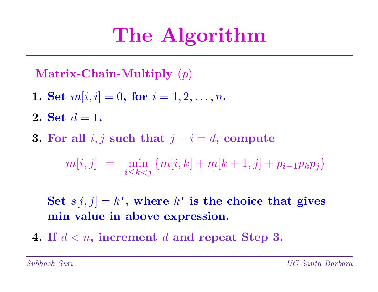
13 . The Algorithm Matrix-Chain-Multiply (p) 1. Set m[i, i] = 0, for i = 1, 2, . . . , n. 2. Set d = 1. 3. For all i, j such that j − i = d, compute m[i, j] = min {m[i, k] + m[k + 1, j] + pi−1pk pj } i≤k<j Set s[i, j] = k ∗, where k ∗ is the choice that gives min value in above expression. 4. If d < n, increment d and repeat Step 3. Subhash Suri UC Santa Barbara
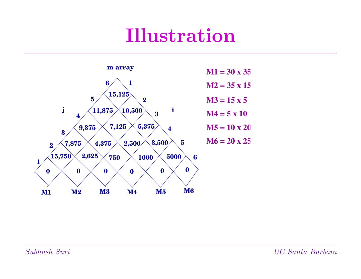
14 . Illustration m array M1 = 30 x 35 6 1 M2 = 35 x 15 15,125 5 2 M3 = 15 x 5 j 11,875 10,500 i 4 3 M4 = 5 x 10 9,375 7,125 5,375 4 M5 = 10 x 20 3 7,875 4,375 2,500 3,500 5 M6 = 20 x 25 2 15,750 2,625 750 1000 5000 6 1 0 0 0 0 0 0 M1 M2 M3 M4 M5 M6 Subhash Suri UC Santa Barbara
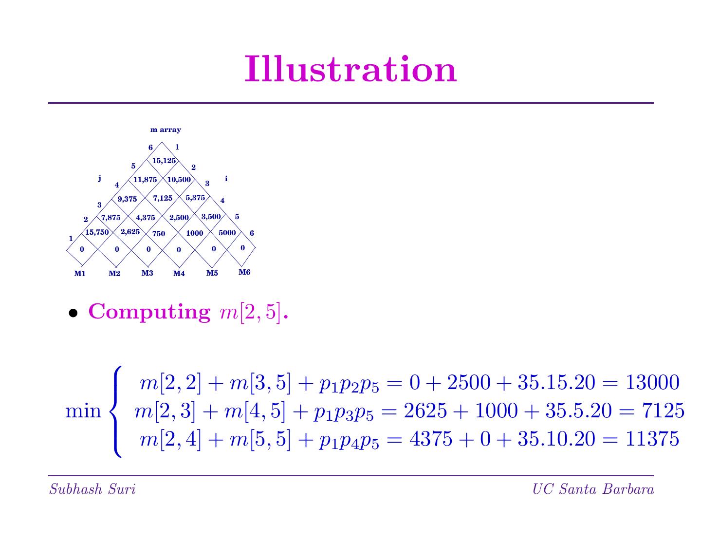
15 . Illustration m array 6 1 15,125 5 2 j 11,875 10,500 i 4 3 9,375 7,125 5,375 4 3 2 7,875 4,375 2,500 3,500 5 15,750 2,625 750 1000 5000 6 1 0 0 0 0 0 0 M1 M2 M3 M4 M5 M6 • Computing m[2, 5]. m[2, 2] + m[3, 5] + p1p2p5 = 0 + 2500 + 35.15.20 = 13000 min m[2, 3] + m[4, 5] + p1p3p5 = 2625 + 1000 + 35.5.20 = 7125 m[2, 4] + m[5, 5] + p1p4p5 = 4375 + 0 + 35.10.20 = 11375 Subhash Suri UC Santa Barbara
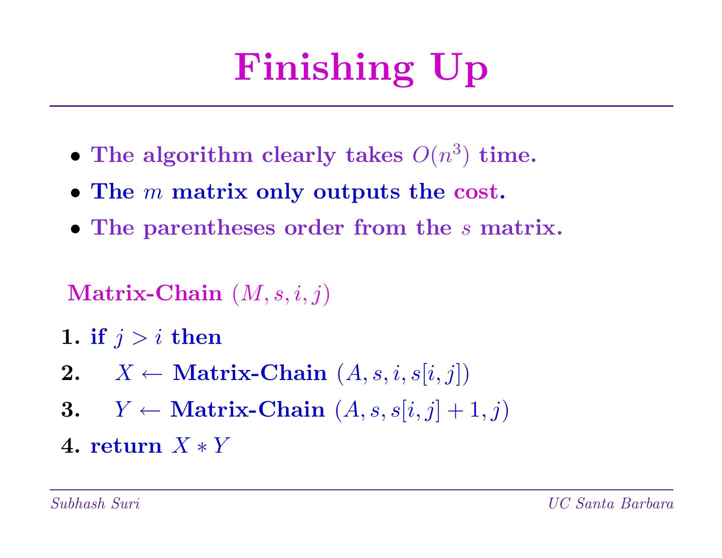
16 . Finishing Up • The algorithm clearly takes O(n3) time. • The m matrix only outputs the cost. • The parentheses order from the s matrix. Matrix-Chain (M, s, i, j) 1. if j > i then 2. X ← Matrix-Chain (A, s, i, s[i, j]) 3. Y ← Matrix-Chain (A, s, s[i, j] + 1, j) 4. return X ∗ Y Subhash Suri UC Santa Barbara
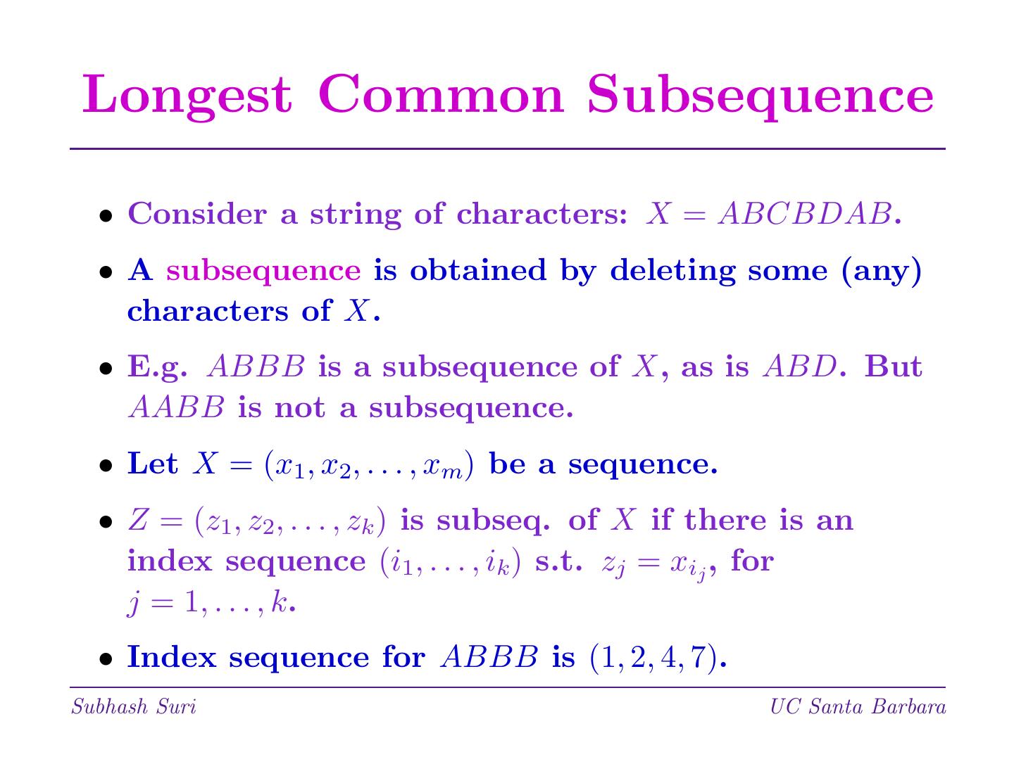
17 . Longest Common Subsequence • Consider a string of characters: X = ABCBDAB. • A subsequence is obtained by deleting some (any) characters of X. • E.g. ABBB is a subsequence of X, as is ABD. But AABB is not a subsequence. • Let X = (x1, x2, . . . , xm) be a sequence. • Z = (z1, z2, . . . , zk ) is subseq. of X if there is an index sequence (i1, . . . , ik ) s.t. zj = xij , for j = 1, . . . , k. • Index sequence for ABBB is (1, 2, 4, 7). Subhash Suri UC Santa Barbara
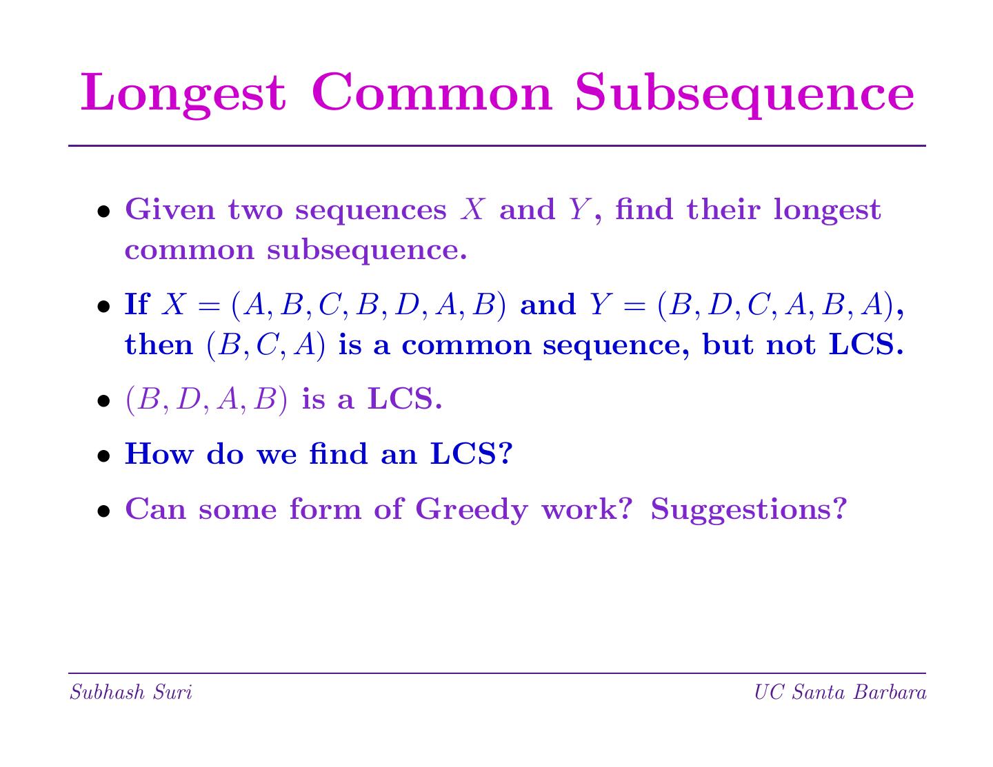
18 . Longest Common Subsequence • Given two sequences X and Y , find their longest common subsequence. • If X = (A, B, C, B, D, A, B) and Y = (B, D, C, A, B, A), then (B, C, A) is a common sequence, but not LCS. • (B, D, A, B) is a LCS. • How do we find an LCS? • Can some form of Greedy work? Suggestions? Subhash Suri UC Santa Barbara
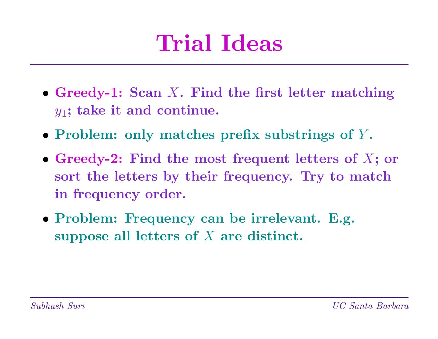
19 . Trial Ideas • Greedy-1: Scan X. Find the first letter matching y1; take it and continue. • Problem: only matches prefix substrings of Y . • Greedy-2: Find the most frequent letters of X; or sort the letters by their frequency. Try to match in frequency order. • Problem: Frequency can be irrelevant. E.g. suppose all letters of X are distinct. Subhash Suri UC Santa Barbara
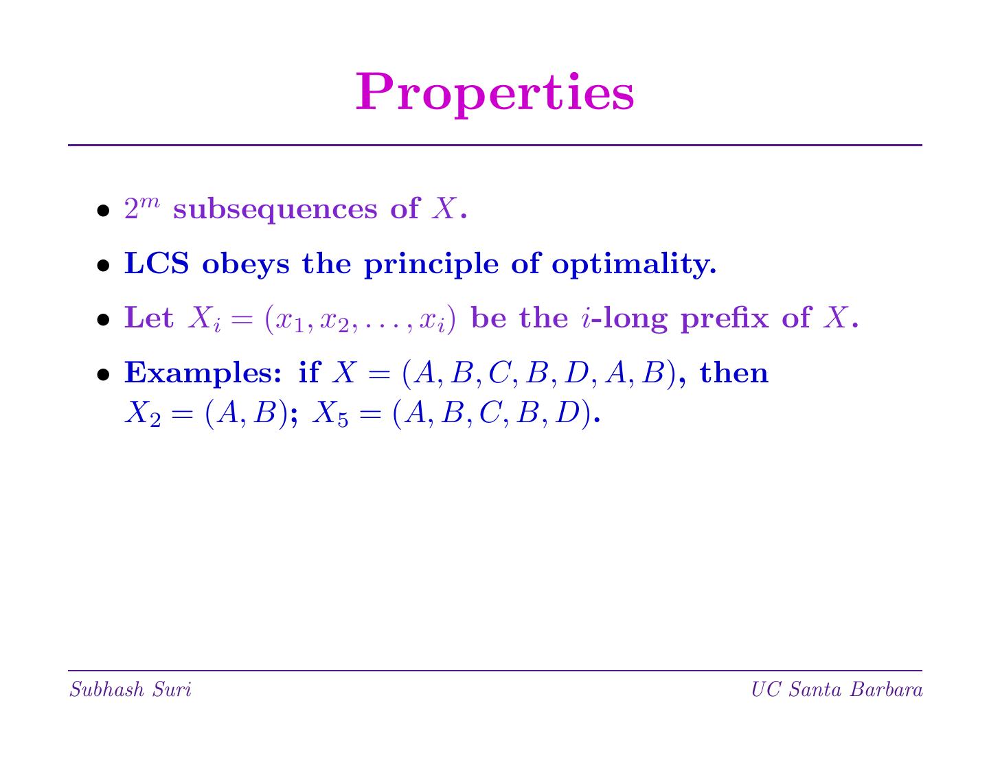
20 . Properties • 2m subsequences of X. • LCS obeys the principle of optimality. • Let Xi = (x1, x2, . . . , xi) be the i-long prefix of X. • Examples: if X = (A, B, C, B, D, A, B), then X2 = (A, B); X5 = (A, B, C, B, D). Subhash Suri UC Santa Barbara
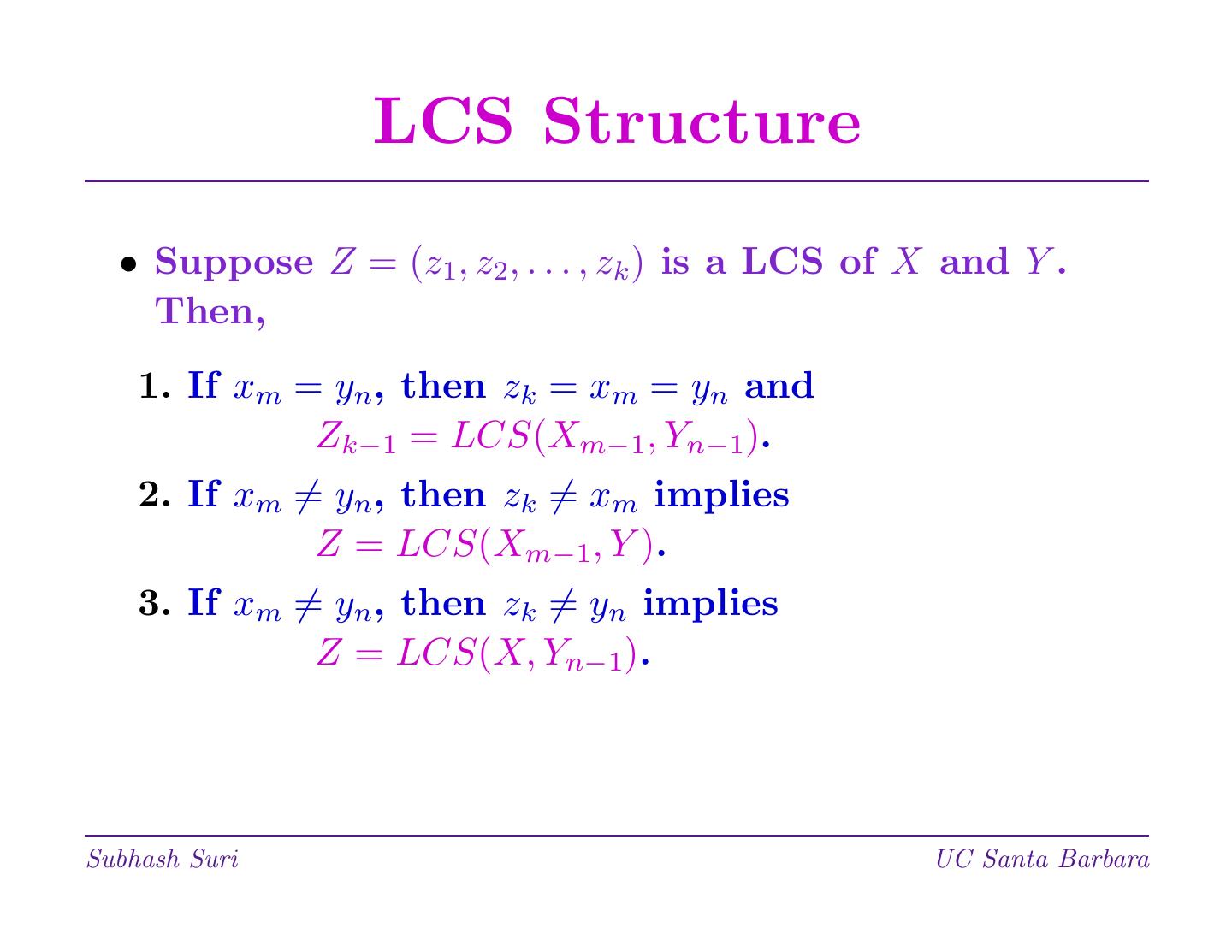
21 . LCS Structure • Suppose Z = (z1, z2, . . . , zk ) is a LCS of X and Y . Then, 1. If xm = yn, then zk = xm = yn and Zk−1 = LCS(Xm−1, Yn−1). 2. If xm = yn, then zk = xm implies Z = LCS(Xm−1, Y ). 3. If xm = yn, then zk = yn implies Z = LCS(X, Yn−1). Subhash Suri UC Santa Barbara
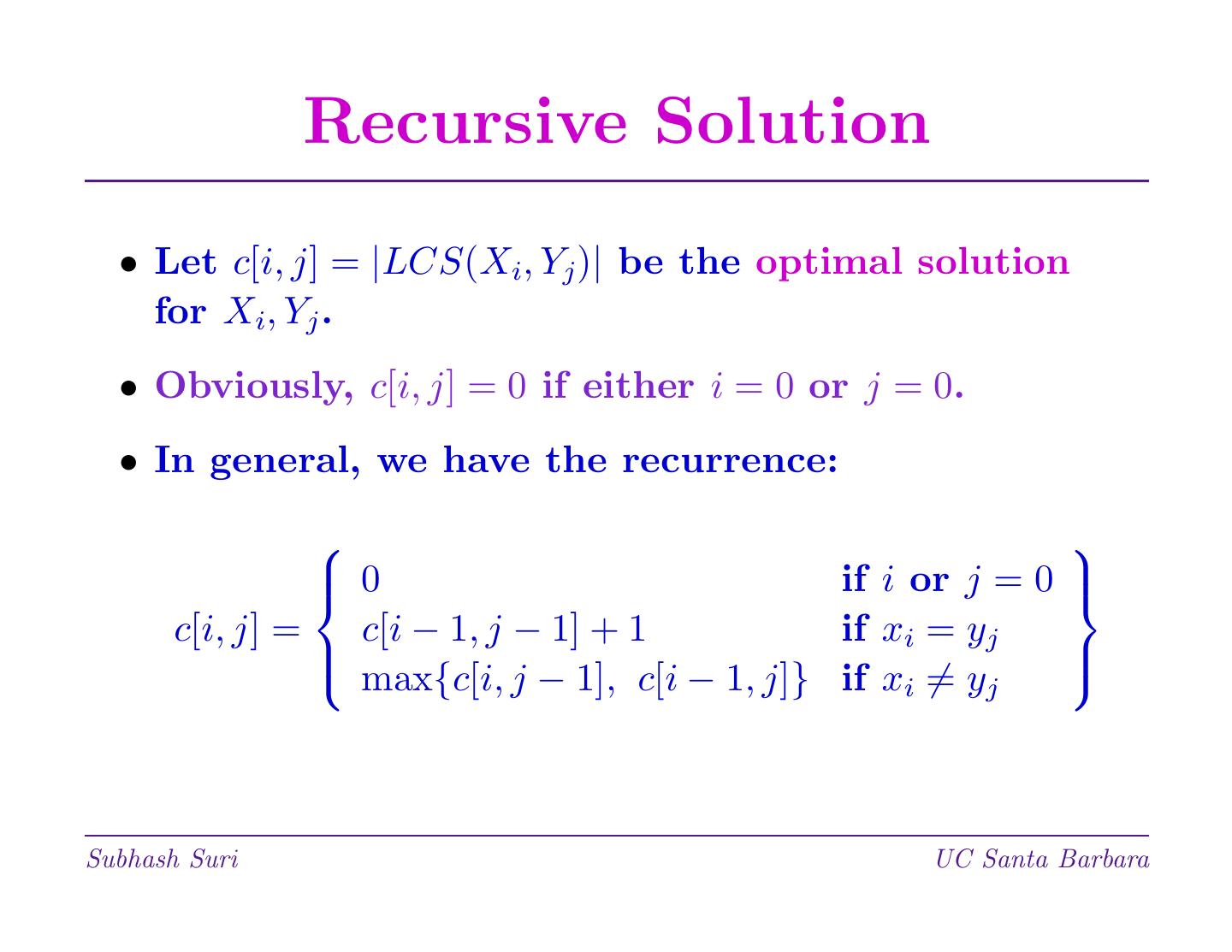
22 . Recursive Solution • Let c[i, j] = |LCS(Xi, Yj )| be the optimal solution for Xi, Yj . • Obviously, c[i, j] = 0 if either i = 0 or j = 0. • In general, we have the recurrence: 0 if i or j = 0 c[i, j] = c[i − 1, j − 1] + 1 if xi = yj max{c[i, j − 1], c[i − 1, j]} if xi = yj Subhash Suri UC Santa Barbara
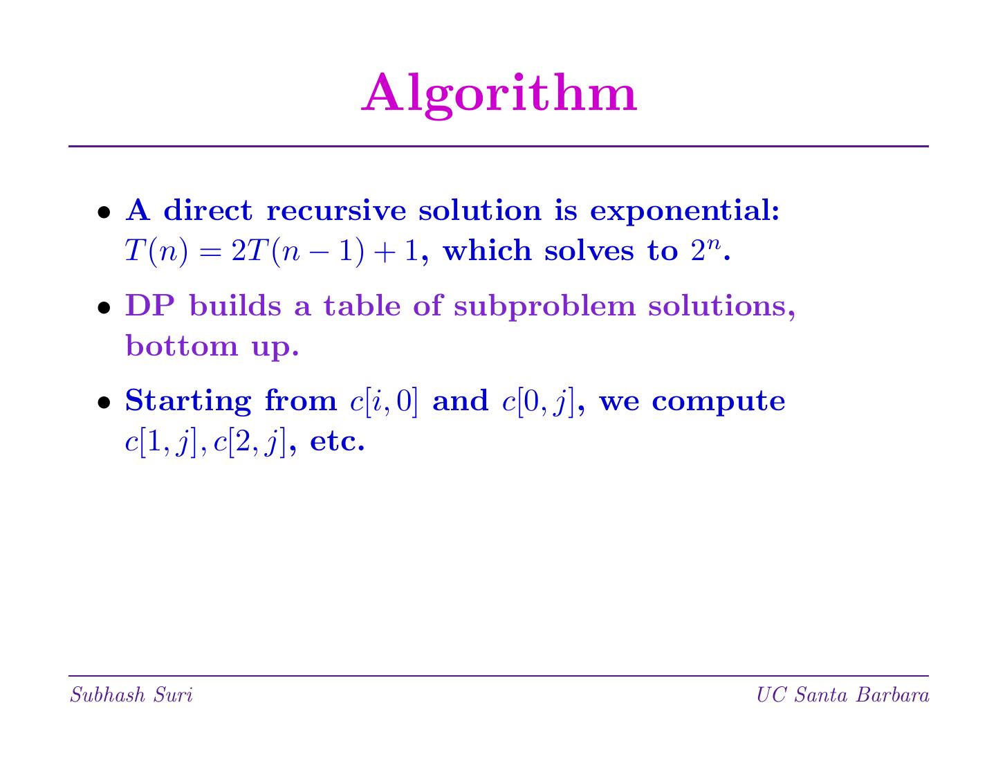
23 . Algorithm • A direct recursive solution is exponential: T (n) = 2T (n − 1) + 1, which solves to 2n. • DP builds a table of subproblem solutions, bottom up. • Starting from c[i, 0] and c[0, j], we compute c[1, j], c[2, j], etc. Subhash Suri UC Santa Barbara
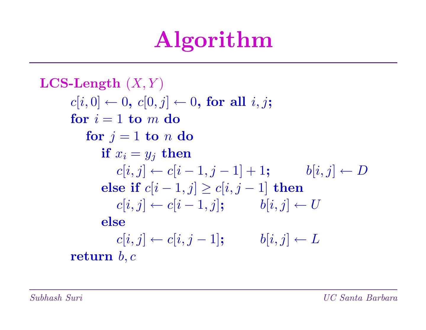
24 . Algorithm LCS-Length (X, Y ) c[i, 0] ← 0, c[0, j] ← 0, for all i, j; for i = 1 to m do for j = 1 to n do if xi = yj then c[i, j] ← c[i − 1, j − 1] + 1; b[i, j] ← D else if c[i − 1, j] ≥ c[i, j − 1] then c[i, j] ← c[i − 1, j]; b[i, j] ← U else c[i, j] ← c[i, j − 1]; b[i, j] ← L return b, c Subhash Suri UC Santa Barbara
25 . LCS Algorithm • LCS-Length (X, Y ) only computes the length of the common subsequence. • By keeping track of matches, xi = yj , the LCS itself can be constructed. Subhash Suri UC Santa Barbara
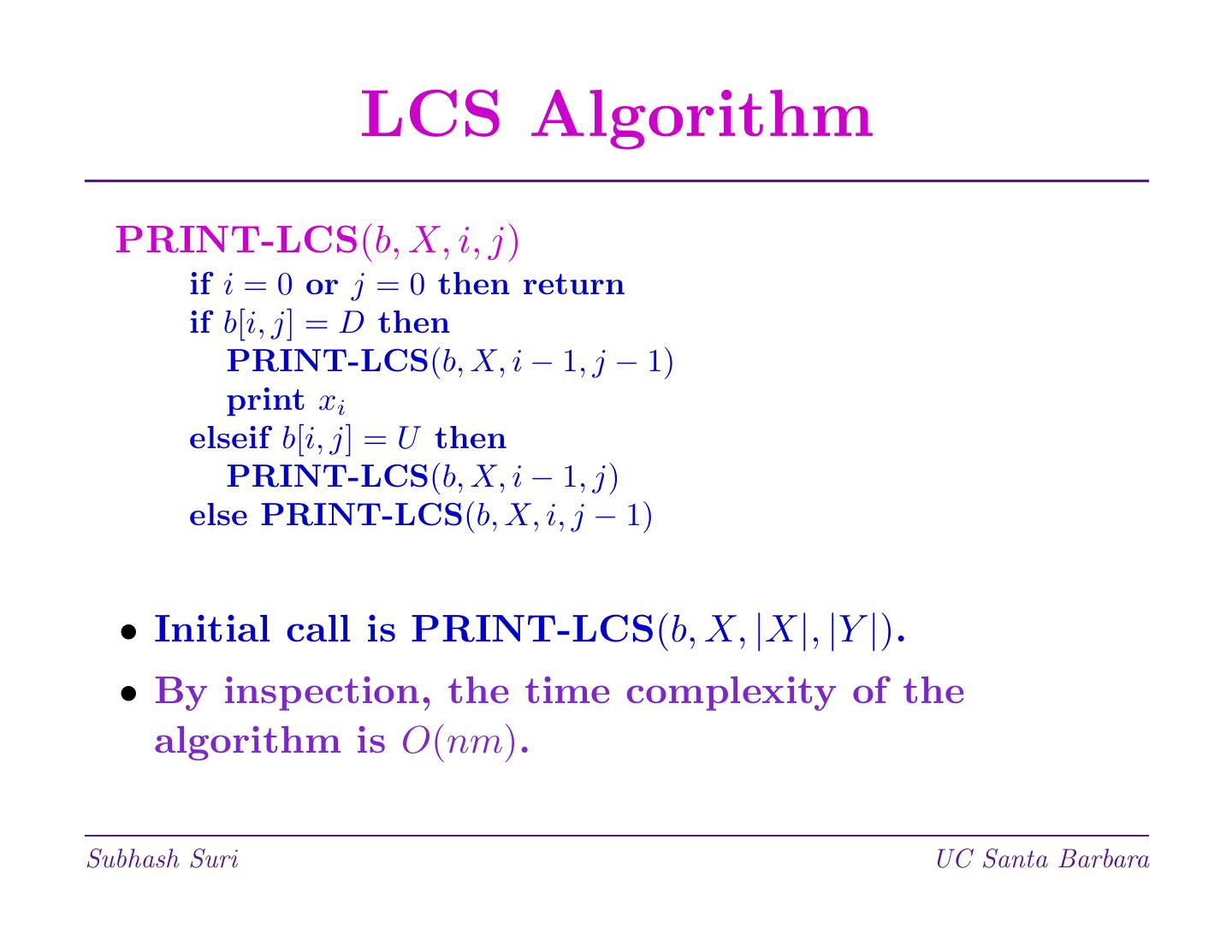
26 . LCS Algorithm PRINT-LCS(b, X, i, j) if i = 0 or j = 0 then return if b[i, j] = D then PRINT-LCS(b, X, i − 1, j − 1) print xi elseif b[i, j] = U then PRINT-LCS(b, X, i − 1, j) else PRINT-LCS(b, X, i, j − 1) • Initial call is PRINT-LCS(b, X, |X|, |Y |). • By inspection, the time complexity of the algorithm is O(nm). Subhash Suri UC Santa Barbara
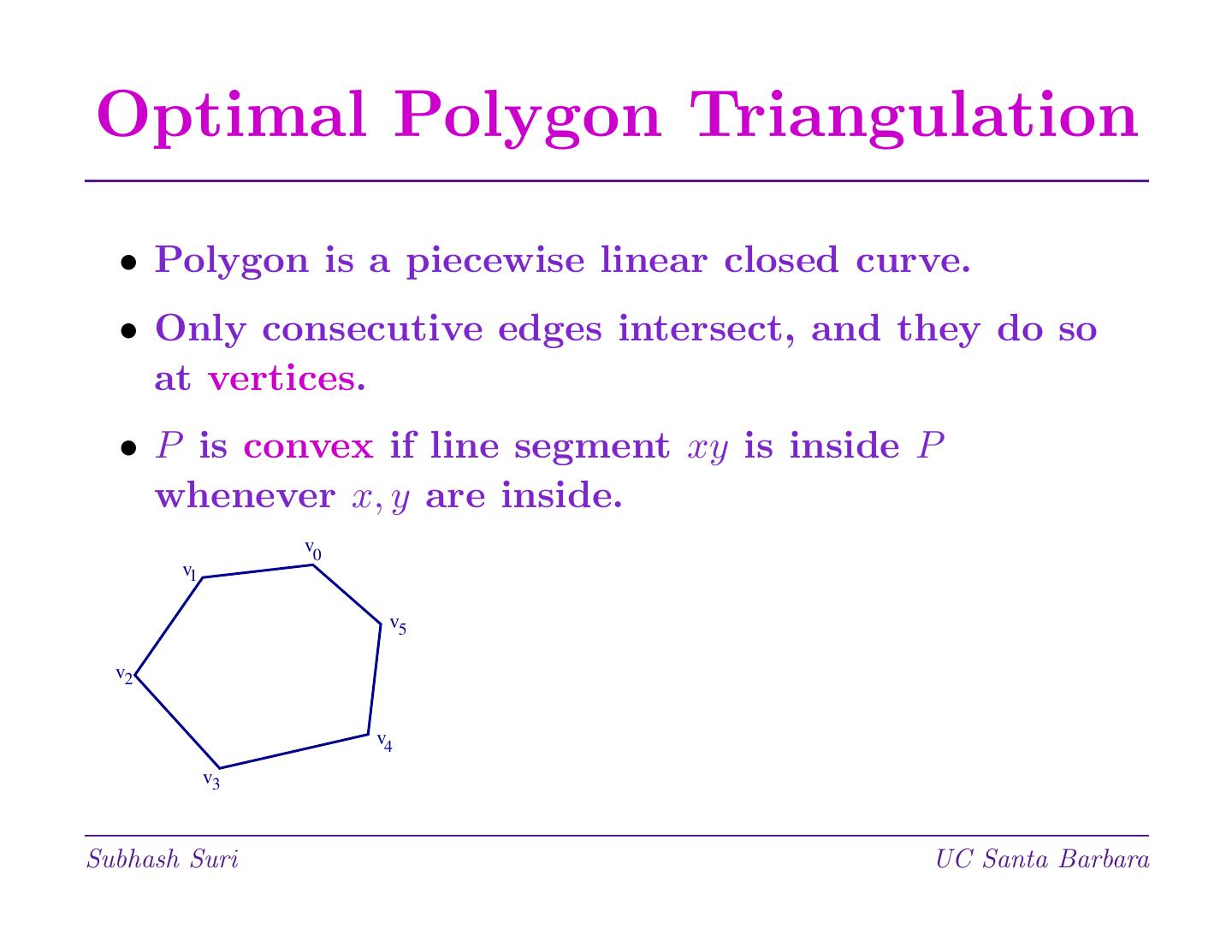
27 .Optimal Polygon Triangulation • Polygon is a piecewise linear closed curve. • Only consecutive edges intersect, and they do so at vertices. • P is convex if line segment xy is inside P whenever x, y are inside. v0 v1 v5 v2 v4 v3 Subhash Suri UC Santa Barbara
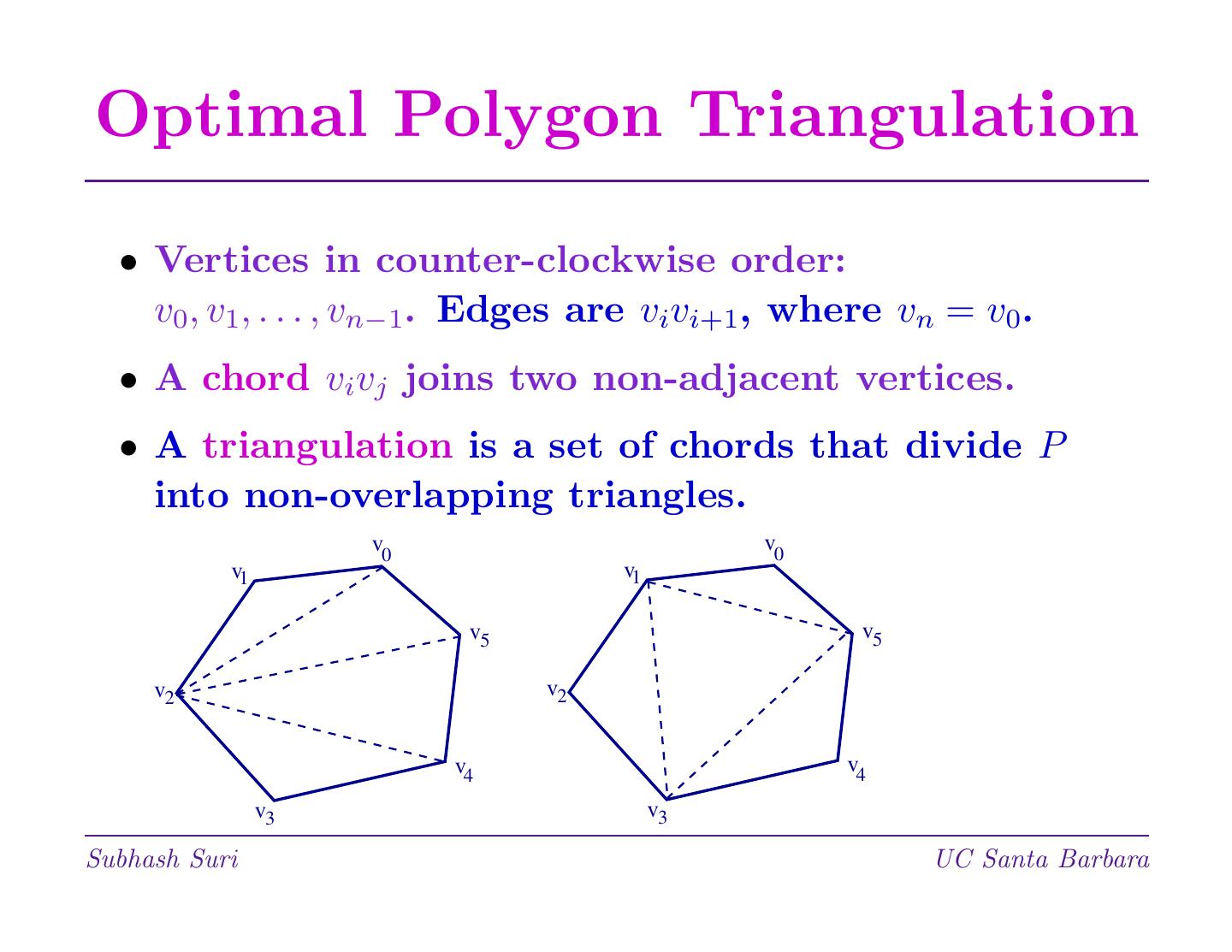
28 .Optimal Polygon Triangulation • Vertices in counter-clockwise order: v0, v1, . . . , vn−1. Edges are vivi+1, where vn = v0. • A chord vivj joins two non-adjacent vertices. • A triangulation is a set of chords that divide P into non-overlapping triangles. v0 v0 v1 v1 v5 v5 v2 v2 v4 v4 v3 v3 Subhash Suri UC Santa Barbara
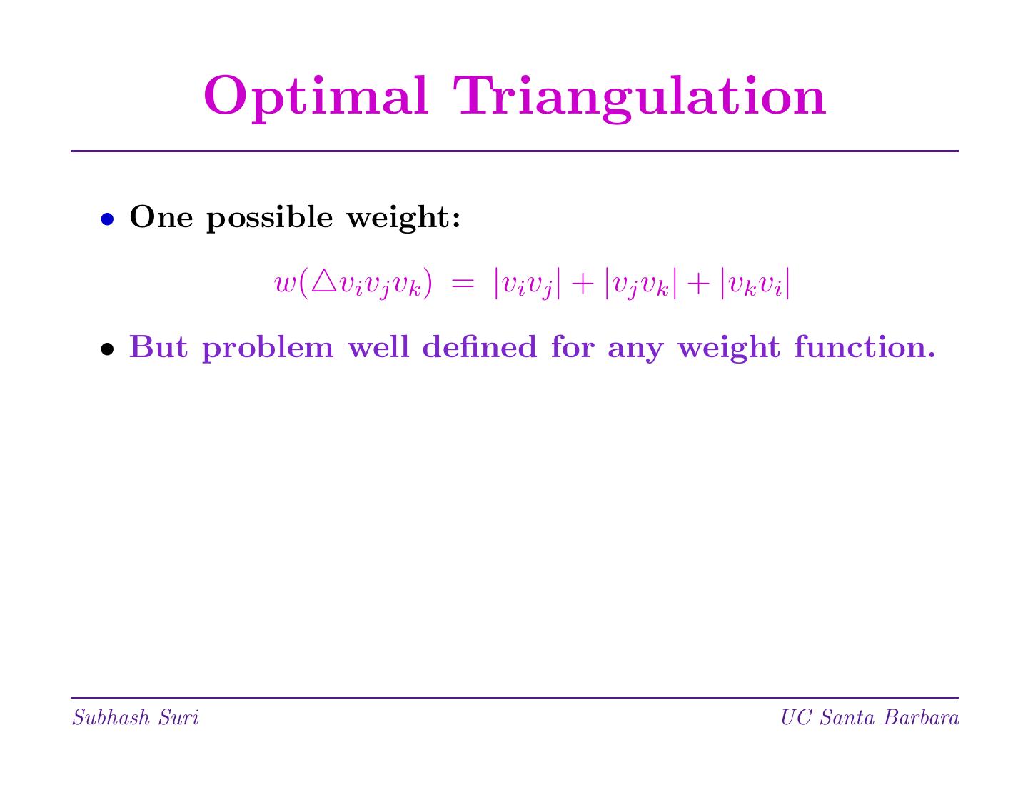
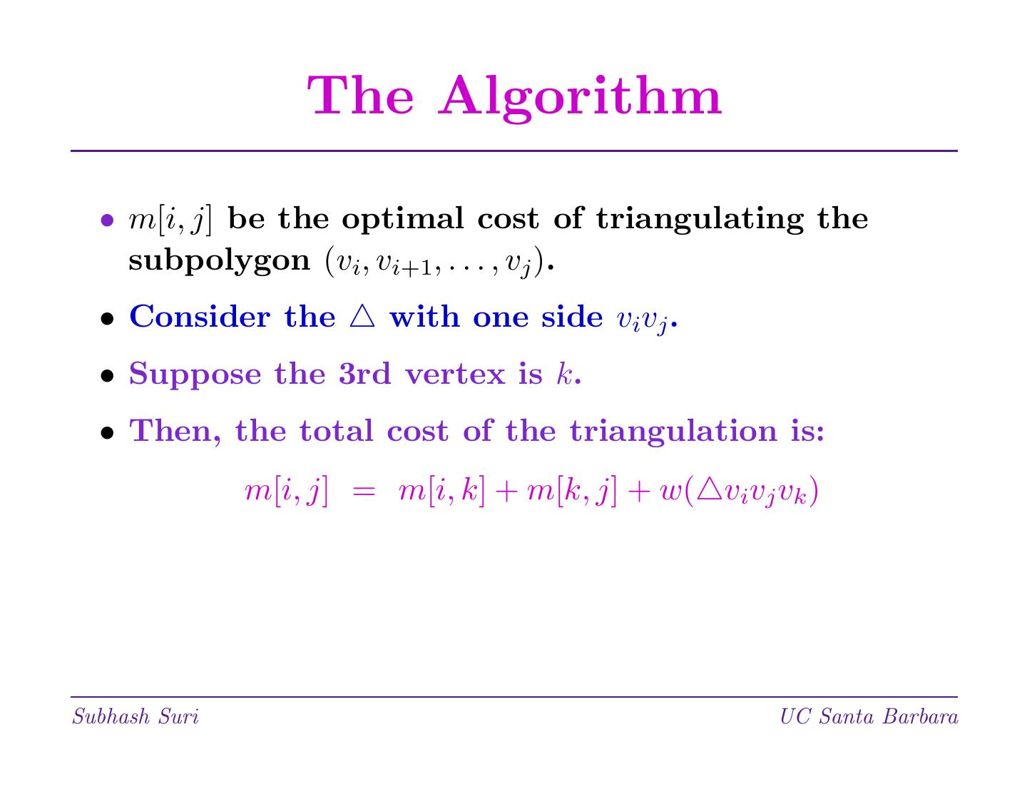
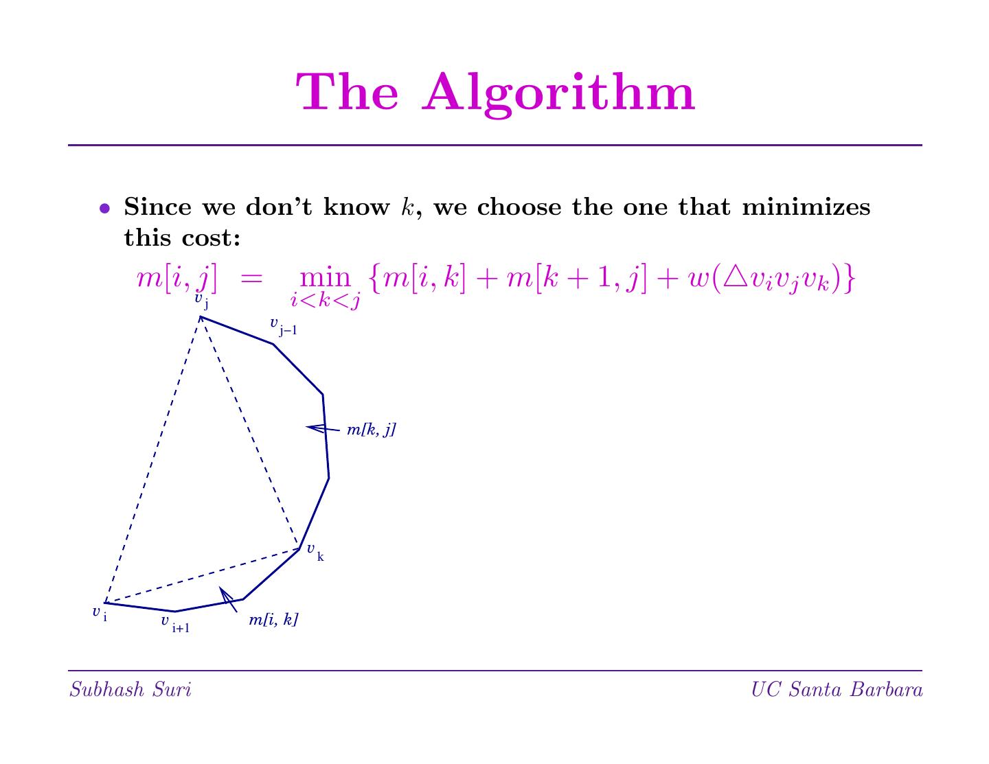
29 . Triangulation Problem • Given a convex polygon P = (v0, . . . , vn−1), and a weight function w on triangles, find a triangulation minimizing the total weight. • Every triangulation of a n-gon has n − 2 triangles and n − 3 chords. v0 v0 v1 v1 v5 v5 v2 v2 v4 v4 v3 v3 Subhash Suri UC Santa Barbara


