Deep Neural Networks (DNN)

1 .Deep Neural Networks (DN N) J.-S. Roger Jang ( 張智星 ) jang@mirlab.org http://mirlab.org/jang MIR Lab, CSIE Dept. National Taiwan University 18年9月2 日 

2 .Concept of Modeling  Modeling  Given desired i/o pairs (training set) of the form (x1, ..., x n; y), construct a model to match the i/o pairs x1 Unknown target system y ... xn Model y*  Two steps in modeling  Structure identification: input selection, model complexit y  Parameter identification: optimal parameters 2/33 

3 .Neural Networks  Supervised Learning  Multilayerperceptrons  Radial basis function networks  Modular neural networks  LVQ (learning vector quantization)  Unsupervised Learning  Competitive learning networks  Kohonen self-organizing networks  ART (adaptive resonant theory)  Others  Hopfield networks 3/33 

4 .Single-layer Perceptrons  Proposed by Widrow & Hoff in 1960  AKA ADALINE (Adaptive Linear Neuron) or single-laye r perceptron Training data x1 x2 (voice freq.) w1 w0 y w2 x2 f  x; w  sgn  w0  w1 x1  w2 x2   1 if female    1 if male Quiz!  w0    y  f  x; w    w1  x1  y  f  x; w  x1 (hair length)  w  x  y  f  x; w  perceptronDemo.m 4/33  2 2 

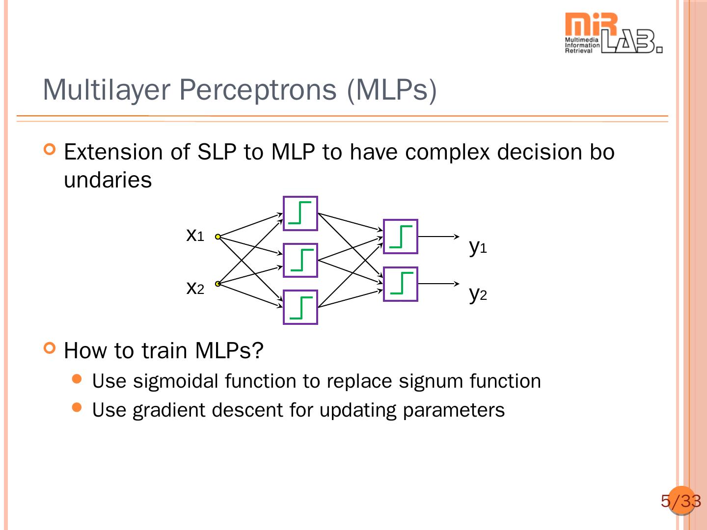
5 .Multilayer Perceptrons (MLPs)  Extension of SLP to MLP to have complex decision bo undaries x1 y1 x2 y2  How to train MLPs?  Use sigmoidal function to replace signum function  Use gradient descent for updating parameters 5/33 

6 .Continuous Activation Functions  In order to use gradient descent, we need to replace the signum function by its continuous versions Sigmoid Hyper-tangent Identity y = 1/(1+exp(-x)) y = tanh(x/2) y=x 6/33 

7 .Activation Functions 1 Sigmoid :   x   1  e x 1  e 2 x Tanh :   x   1  e 2 x x Softsign :   x   1 x  x if x  0 ReLU :   x     0 otherwise  x if x  0 Leaky ReLU :   x     x otherwise Softplus :   x   ln 1  e x  7/33 

8 .Classical MLPs  Typical 2-layer MLPs: x1 y1 x2 y2  Learning rule  Gradient descent (Backpropagation)  Conjugate gradient method  All optim. methods using first derivative  Derivative-free optim. 8/33 

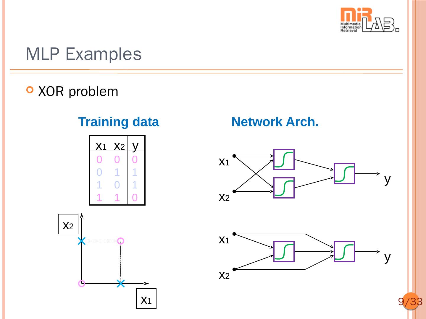
9 .MLP Examples  XOR problem Training data Network Arch. x1 x2 y 0 0 0 x1 0 1 1 1 0 1 y 1 1 0 x2 x2 x1 y x2 x1 9/33 

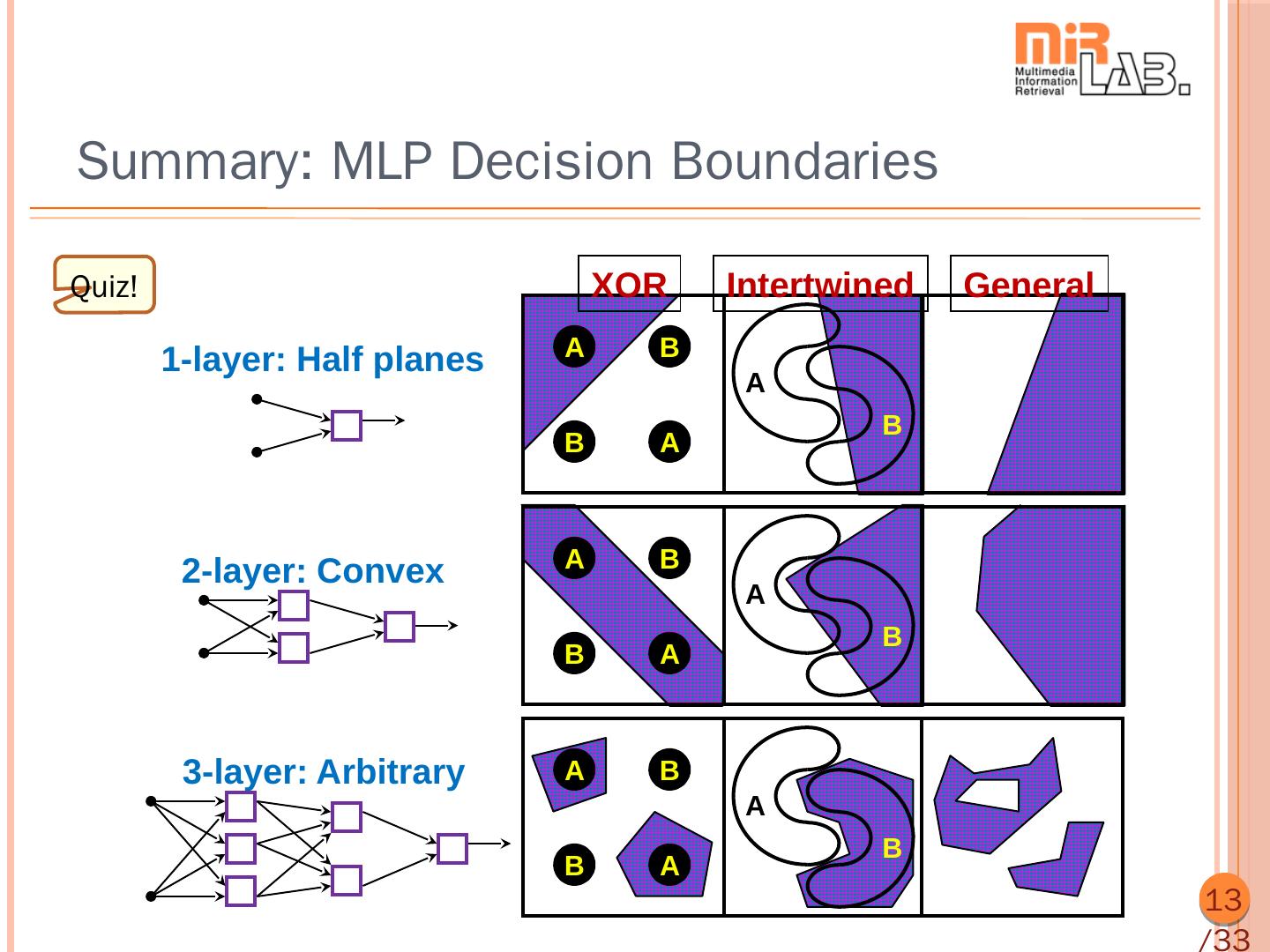
10 .MLP Decision Boundaries  Single-layer: Half planes Exclusive-OR Meshed Most general problem regions regions A B A B B A 10 /33 

11 .MLP Decision Boundaries  Two-layer: Convex regions Exclusive-OR Meshed Most general problem regions regions A B A B B A 11 /33 

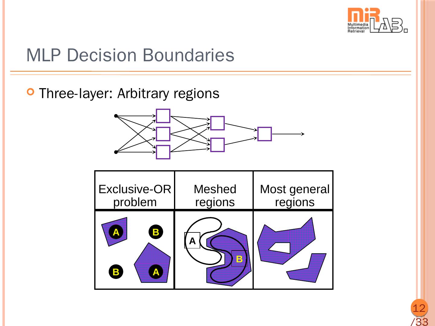
12 .MLP Decision Boundaries  Three-layer: Arbitrary regions Exclusive-OR Meshed Most general problem regions regions A B A B B A 12 /33 

13 .Summary: MLP Decision Boundaries Quiz! XOR Intertwined General A B 1-layer: Half planes A B B A 2-layer: Convex A B A B B A 3-layer: Arbitrary A B A B B A 13 /33 

14 .MLP Configurations 14 /33 

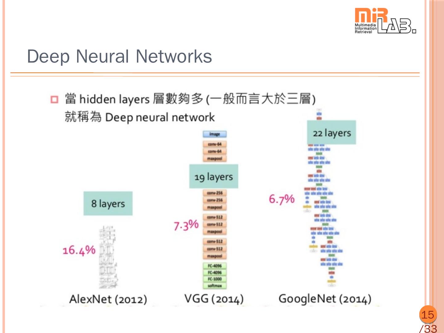
15 .Deep Neural Networks 15 /33 

16 .Training an MLP  Methods for training MLP  Gradientdescent  Gauss-Newton method  Levenberg-Marquart method  Backpropagation: A systematic way to compute grad ients, starting from the NN’s output Training set :   x i , yi  | i  1,2,  , n Model : y  f  x, θ  n Sum of squared error : E (θ)    yi  f  x i , θ   2 i 1 n E (θ)    2 yi  f  x i , θ    θ f  x i , θ  i 1 16 /33 

17 .Simple Derivatives  Review of chain rule dy df  x  y df  x  y  f  x     dx dx x dx  Network representation x f(.) y 17 /33 

18 .Chain Rule for Composite Functions  Review of chain rule  y  f  x dz dz dy dg  y  df  x    z  g f  x      z  g y dx dy dx dy dx  Network representation y x f(.) g(.) z 18 /33 

19 .Chain Rule for Network Representation  Review of chain rule  y  f  x  du u dy u dz  z  g  x  u  h  f  x  , g  x       u  h y , z  dx y dx z dx   Network representation y f(.) h(. , x .) u g(, ) z 19 /33 

20 .Backpropagation in Adaptive Networks (1/ 3)  Backpropagation A way to compute gradient from output toward input  Adaptive network  Node 1 : u  x  ey   Node 2 : v  ln   x  y  u x 1     Node 3 : o  u 2  v 3 /  Network input : x, y 3 o Network output : o y 2 Network parameters :  ,  ,  v Overall function : o  f ( x,y ; α,β,γ  ) output inputs parameters 20 /33 

21 .Backpropagation in Adaptive Networks (2/ 3) x 1 u 3 o y 2 v  Node 1 : u  x  ey   Node 2 : v  ln  x  y    Node 3 : o  u 2  v 3 /    21 /33 

22 . Backpropagation in Adaptive Networks (3/ 3) x 1 P 3 u 5 o y 2 q 4 v  Node 1 : p  x  ey   Node 2 : q  ln  x  y     Node 3 : u  p  q /  2 3   Node 4 : v  pq    Node 5 : o  u ln v  v ln u You don’t need to ! 22 /33 

23 .Summary of Backpropagation  General formula for backpropagation, assuming  “o” is the network’s final output  “” is a parameter in node 1  o o x Backpropagation! y1    x   o o y o y2 o y3   1   x  x y1 x y2 x y3 x y2 o o o 1 , , : Derivatives in the next layer y1 y2 y3 y3 y1 y2 y3 , , : Weights of backpropagation  x x x 23 /33 

24 . Backpropagation in NN (1/2) x1 1 y1 1 o x2 2 y2  1  1 y     x   x     1  e (11 x1 12 x2 1 ) 11 1 12 2 1   1  y2     21 x1   22 x2   2    ( 21 x1  22 x2  2 )  1  e  1  o     y   y     1  e ( 11 y1  12 y2  1 ) 11 1 12 2 1  25 /33 

25 . Backpropagation in NN (2/2) x1 1 y1 1 z1 x2 2 1 o y2 2 z2 x3 3 y3  1 y  i     x   x   x     1  e ( i1 x1  i 2 x2  i 3 x3  i ) i1 1 i2 2 i3 3 i   1  zi     i1 y1   i 2 y2   i 3 y3   i    1  e ( i1 y1  i 2 y2  i 3 y3  i )  1  o     z   z     26 1  e ( 11 z1  12 z2  1 ) 11 1 12 2 1  /33 

26 .Use of Mini-batch in Gradient Descent  Goal: To speed up the training with large dataset A process of going through all data  Approach: Update by mini-batch instead of epoch  If dataset size is 1000  Batch size = 10  100 updates in an epoch  mini bat ch  Batch size = 100  10 updates in an epoch  mini bat ch Update by epoch  Batch size=1000 Update  1 update in by mini-batch an epoch  full batch Slower Faster update! update! 27 /33 

27 .Use of Momentum Term in Gradient Desc ent  Purpose of using momentum term  Avoidoscillations in gradient descent (banana function!)  Escape from local minima (???)  Formula  Original: θ  E  θ  Contours of banana function  Withmomentum term: θ  E  θ     θ  prev Momentum term 28 /33 

28 .Learning Rate Selection 29 /33 

29 .Optimizer in Keras  Choices of optimization methods in Keras  SGD: Stochastic gradient descent  Adagrad: Adaptive learning rate  RMSprop: Similar to Adagrad  Adam: Similar to RMSprop + momentum  Nadam: Adam + Nesterov momentum 30 /33