logistic regression

1 .Logistic Regression Logistic Regression Jia Li Department of Statistics The Pennsylvania State University Email: jiali@stat.psu.edu http://www.stat.psu.edu/∼jiali Jia Li http://www.stat.psu.edu/∼jiali 

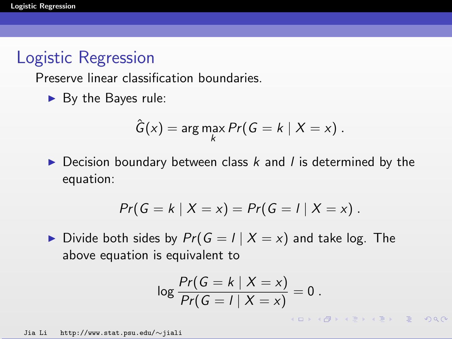
2 .Logistic Regression Logistic Regression Preserve linear classification boundaries. By the Bayes rule: ˆ (x) = arg max Pr (G = k | X = x) . G k Decision boundary between class k and l is determined by the equation: Pr (G = k | X = x) = Pr (G = l | X = x) . Divide both sides by Pr (G = l | X = x) and take log. The above equation is equivalent to Pr (G = k | X = x) log =0. Pr (G = l | X = x) Jia Li http://www.stat.psu.edu/∼jiali 

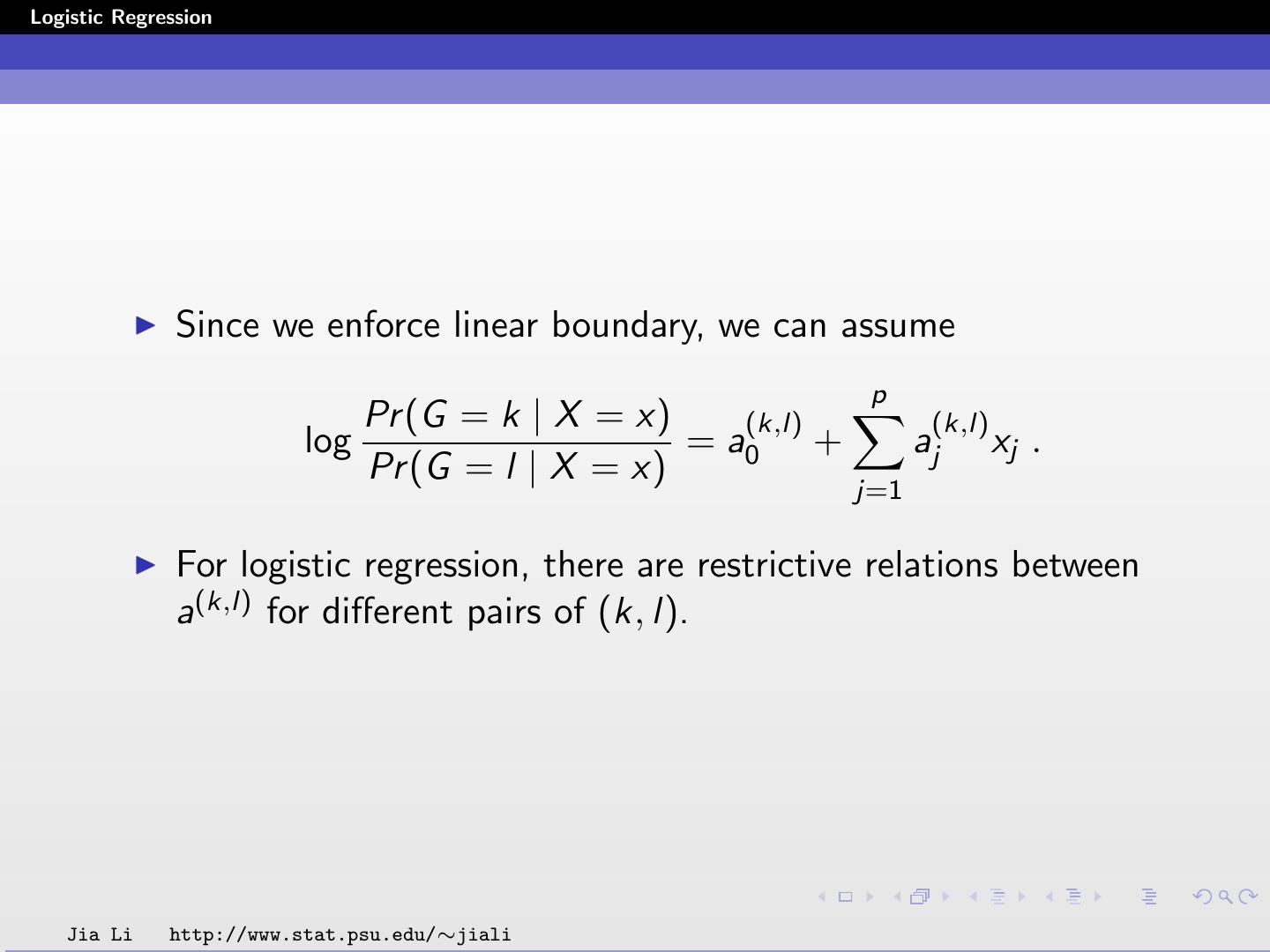
3 .Logistic Regression Since we enforce linear boundary, we can assume p Pr (G = k | X = x) (k,l) (k,l) log = a0 + aj xj . Pr (G = l | X = x) j=1 For logistic regression, there are restrictive relations between a(k,l) for different pairs of (k, l). Jia Li http://www.stat.psu.edu/∼jiali 

4 .Logistic Regression Assumptions Pr (G = 1 | X = x) log = β10 + β1T x Pr (G = K | X = x) Pr (G = 2 | X = x) log = β20 + β2T x Pr (G = K | X = x) .. . Pr (G = K − 1 | X = x) log = β(K −1)0 + βKT −1 x Pr (G = K | X = x) Jia Li http://www.stat.psu.edu/∼jiali 

5 .Logistic Regression For any pair (k, l): Pr (G = k | X = x) log = βk0 − βl0 + (βk − βl )T x . Pr (G = l | X = x) Number of parameters: (K − 1)(p + 1). Denote the entire parameter set by θ = {β10 , β1 , β20 , β2 , ..., β(K −1)0 , βK −1 } . The log ratio of posterior probabilities are called log-odds or logit transformations. Jia Li http://www.stat.psu.edu/∼jiali 

6 .Logistic Regression Under the assumptions, the posterior probabilities are given by: exp(βk0 + βkT x) Pr (G = k | X = x) = K −1 1+ l=1 exp(βl0 + βlT x) for k = 1, ..., K − 1 1 Pr (G = K | X = x) = K −1 . 1+ l=1 exp(βl0 + βlT x) For Pr (G = k | X = x) given above, obviously K Sum up to 1: k=1 Pr (G = k | X = x) = 1. A simple calculation shows that the assumptions are satisfied. Jia Li http://www.stat.psu.edu/∼jiali 

7 .Logistic Regression Comparison with LR on Indicators Similarities: Both attempt to estimate Pr (G = k | X = x). Both have linear classification boundaries. Difference: Linear regression on indicator matrix: approximate Pr (G = k | X = x) by a linear function of x. Pr (G = k | X = x) is not guaranteed to fall between 0 and 1 and to sum up to 1. Logistic regression: Pr (G = k | X = x) is a nonlinear function of x. It is guaranteed to range from 0 to 1 and to sum up to 1. Jia Li http://www.stat.psu.edu/∼jiali 

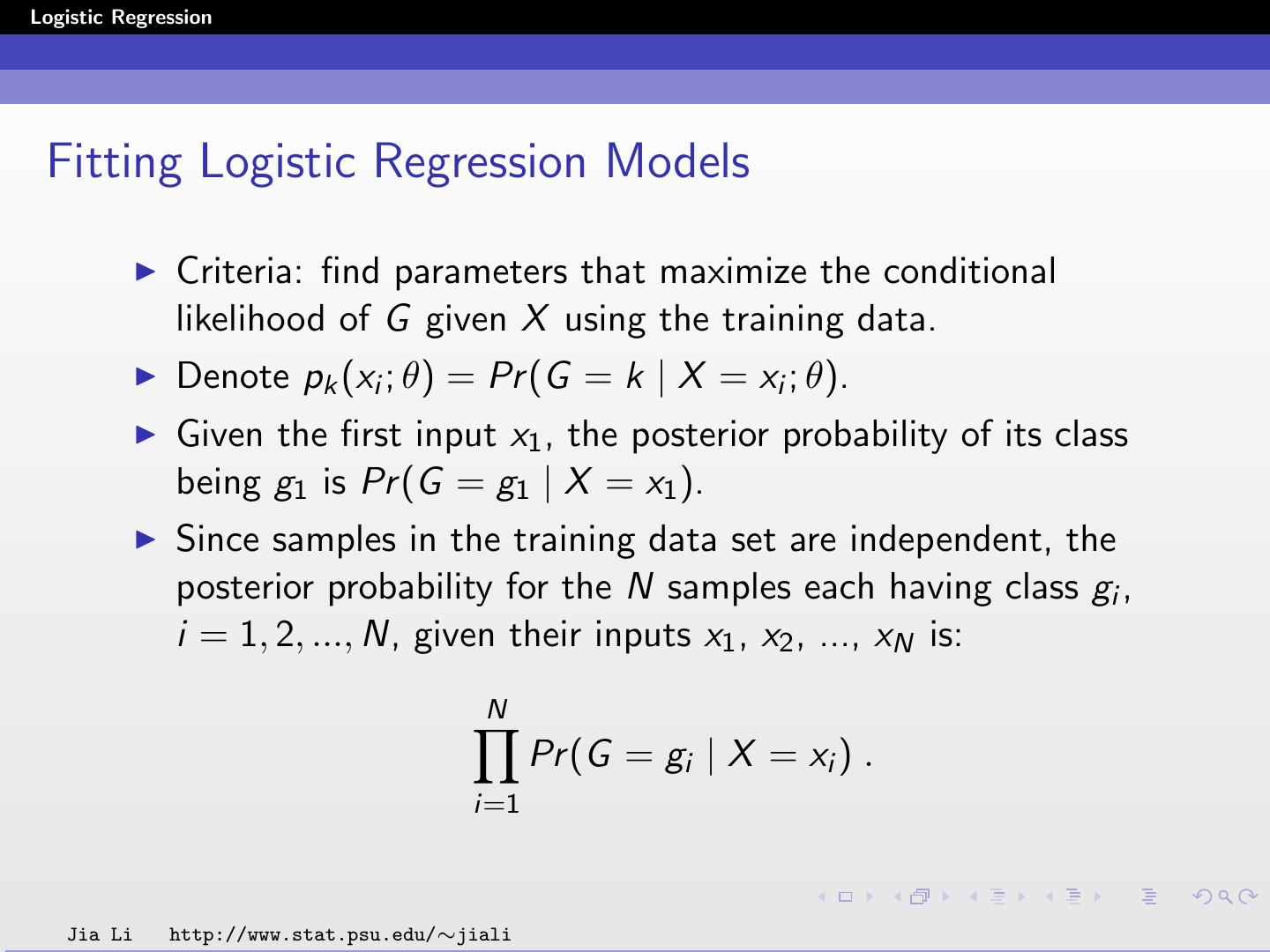
8 .Logistic Regression Fitting Logistic Regression Models Criteria: find parameters that maximize the conditional likelihood of G given X using the training data. Denote pk (xi ; θ) = Pr (G = k | X = xi ; θ). Given the first input x1 , the posterior probability of its class being g1 is Pr (G = g1 | X = x1 ). Since samples in the training data set are independent, the posterior probability for the N samples each having class gi , i = 1, 2, ..., N, given their inputs x1 , x2 , ..., xN is: N Pr (G = gi | X = xi ) . i=1 Jia Li http://www.stat.psu.edu/∼jiali 

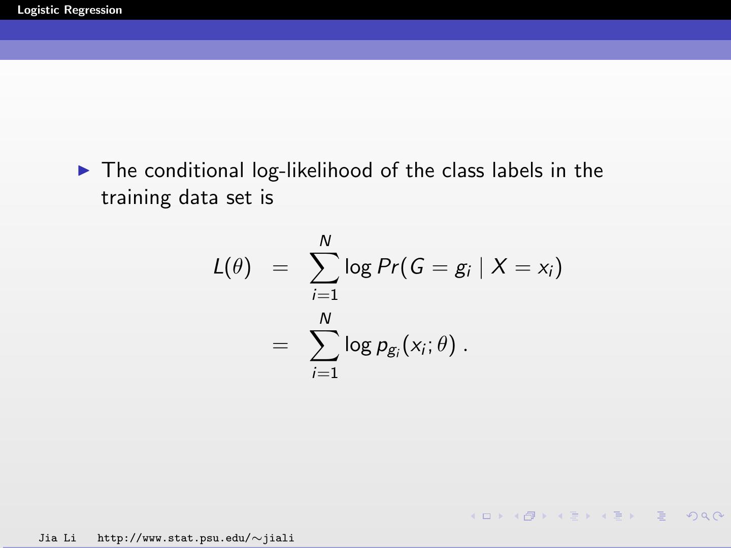
9 .Logistic Regression The conditional log-likelihood of the class labels in the training data set is N L(θ) = log Pr (G = gi | X = xi ) i=1 N = log pgi (xi ; θ) . i=1 Jia Li http://www.stat.psu.edu/∼jiali 

10 .Logistic Regression Binary Classification For binary classification, if gi = 1, denote yi = 1; if gi = 2, denote yi = 0. Let p1 (x; θ) = p(x; θ), then p2 (x; θ) = 1 − p1 (x; θ) = 1 − p(x; θ) . Since K = 2, the parameters θ = {β10 , β1 }. We denote β = (β10 , β1 )T . Jia Li http://www.stat.psu.edu/∼jiali 

11 .Logistic Regression If yi = 1, i.e., gi = 1, log pgi (x; β) = log p1 (x; β) = 1 · log p(x; β) = yi log p(x; β) . If yi = 0, i.e., gi = 2, log pgi (x; β) = log p2 (x; β) = 1 · log(1 − p(x; β)) = (1 − yi ) log(1 − p(x; β)) . Since either yi = 0 or 1 − yi = 0, we have log pgi (x; β) = yi log p(x; β) + (1 − yi ) log(1 − p(x; β)) . Jia Li http://www.stat.psu.edu/∼jiali 

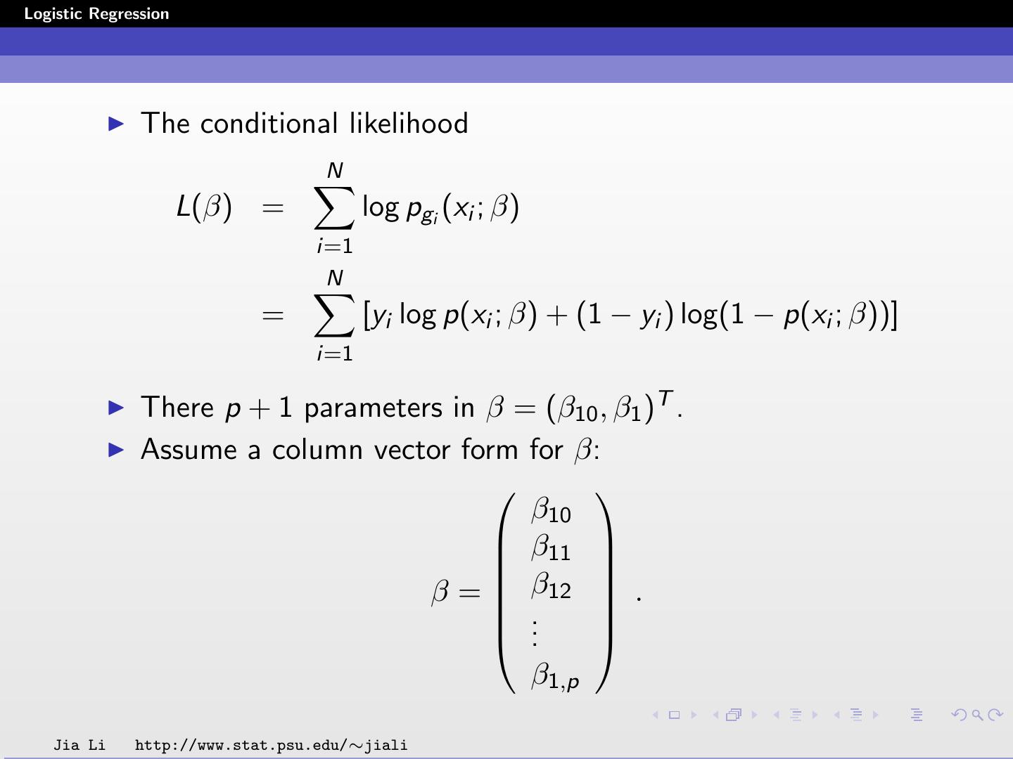
12 .Logistic Regression The conditional likelihood N L(β) = log pgi (xi ; β) i=1 N = [yi log p(xi ; β) + (1 − yi ) log(1 − p(xi ; β))] i=1 There p + 1 parameters in β = (β10 , β1 )T . Assume a column vector form for β:   β10  β11    β =  β12  .    ..   .  β1,p Jia Li http://www.stat.psu.edu/∼jiali 

13 .Logistic Regression Here we add the constant term 1 to x to accommodate the intercept.   1  x,1    x =  x,2  .    ..   .  x,p Jia Li http://www.stat.psu.edu/∼jiali 

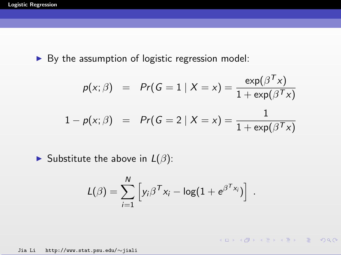
14 .Logistic Regression By the assumption of logistic regression model: exp(β T x) p(x; β) = Pr (G = 1 | X = x) = 1 + exp(β T x) 1 1 − p(x; β) = Pr (G = 2 | X = x) = 1 + exp(β T x) Substitute the above in L(β): N Tx L(β) = yi β T xi − log(1 + e β i ) . i=1 Jia Li http://www.stat.psu.edu/∼jiali 

15 .Logistic Regression To maximize L(β), we set the first order partial derivatives of L(β) to zero. N N T ∂L(β) xij e β xi = yi xij − β1j i=1 i=1 1 + e β T xi N N = yi xij − p(x; β)xij i=1 i=1 N = xij (yi − p(xi ; β)) i=1 for all j = 0, 1, ..., p. Jia Li http://www.stat.psu.edu/∼jiali 

16 .Logistic Regression In matrix form, we write N ∂L(β) = xi (yi − p(xi ; β)) . ∂β i=1 To solve the set of p + 1 nonlinear equations ∂L(β) ∂β1j = 0, j = 0, 1, ..., p, use the Newton-Raphson algorithm. The Newton-Raphson algorithm requires the second-derivatives or Hessian matrix: N ∂ 2 L(β) =− xi xiT p(xi ; β)(1 − p(xi ; β)) . ∂β∂β T i=1 Jia Li http://www.stat.psu.edu/∼jiali 

17 .Logistic Regression The element on the jth row and nth column is (counting from 0): ∂L(β) ∂β1j ∂β1n N Tx T Tx (1 + e β i )e β xi xij xin − (e β i )2 xij xin = − i=1 (1 + e β T xi )2 N = − xij xin p(xi ; β) − xij xin p(xi ; β)2 i=1 N = − xij xin p(xi ; β)(1 − p(xi ; β)) . i=1 Jia Li http://www.stat.psu.edu/∼jiali 

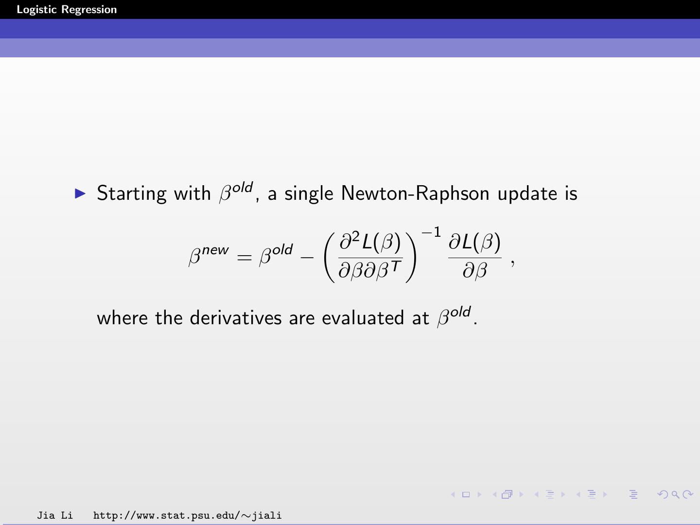
18 .Logistic Regression Starting with β old , a single Newton-Raphson update is −1 new old ∂ 2 L(β) ∂L(β) β =β − , ∂β∂β T ∂β where the derivatives are evaluated at β old . Jia Li http://www.stat.psu.edu/∼jiali 

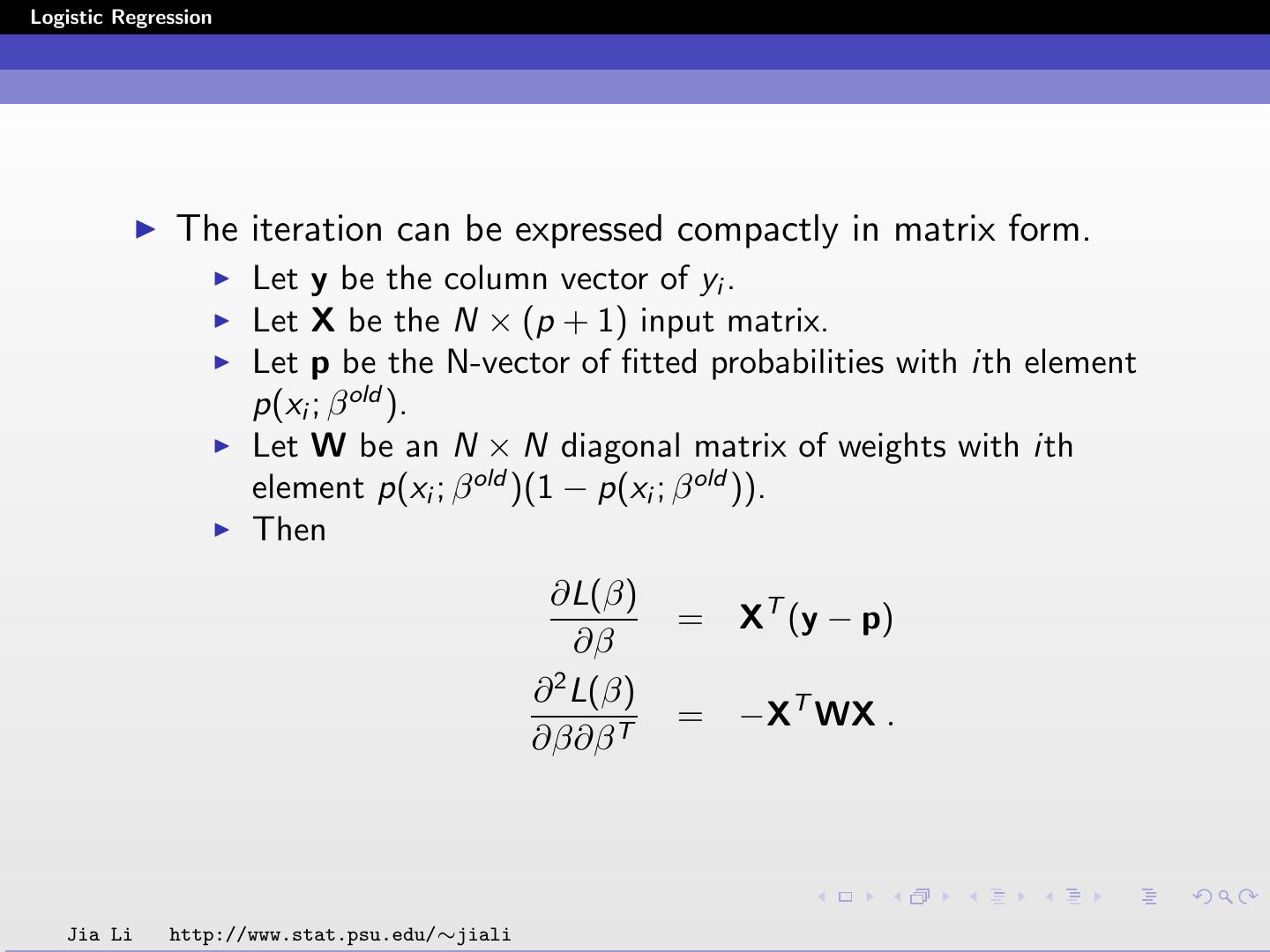
19 .Logistic Regression The iteration can be expressed compactly in matrix form. Let y be the column vector of yi . Let X be the N × (p + 1) input matrix. Let p be the N-vector of fitted probabilities with ith element p(xi ; β old ). Let W be an N × N diagonal matrix of weights with ith element p(xi ; β old )(1 − p(xi ; β old )). Then ∂L(β) = XT (y − p) ∂β 2 ∂ L(β) = −XT WX . ∂β∂β T Jia Li http://www.stat.psu.edu/∼jiali 

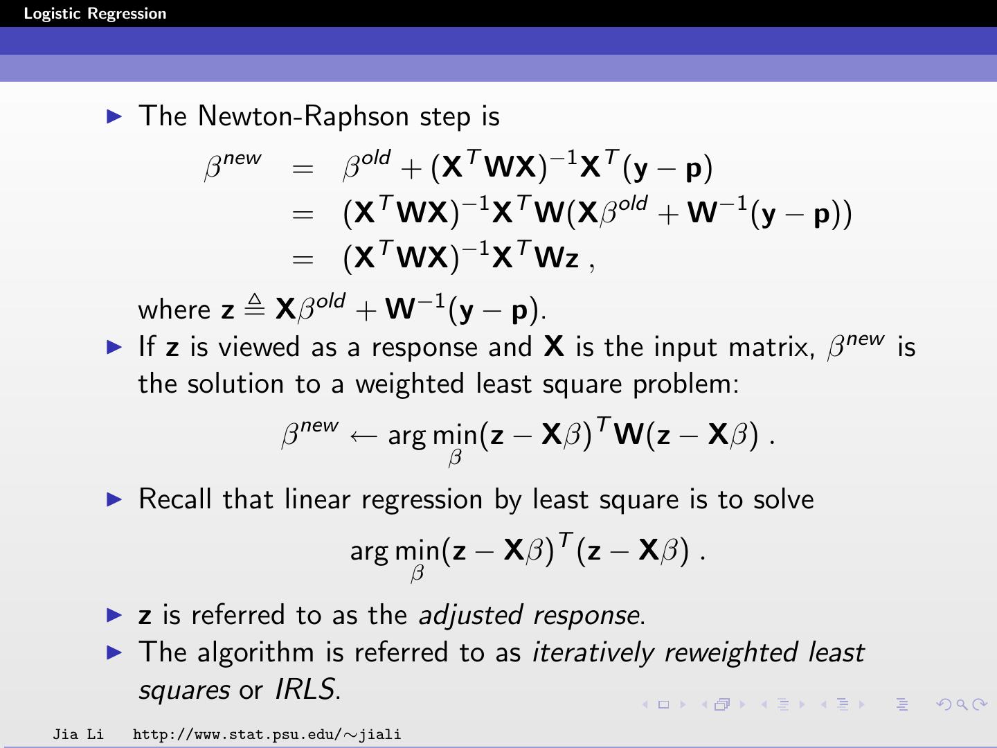
20 .Logistic Regression The Newton-Raphson step is β new = β old + (XT WX)−1 XT (y − p) = (XT WX)−1 XT W(Xβ old + W−1 (y − p)) = (XT WX)−1 XT Wz , where z Xβ old + W−1 (y − p). If z is viewed as a response and X is the input matrix, β new is the solution to a weighted least square problem: β new ← arg min(z − Xβ)T W(z − Xβ) . β Recall that linear regression by least square is to solve arg min(z − Xβ)T (z − Xβ) . β z is referred to as the adjusted response. The algorithm is referred to as iteratively reweighted least squares or IRLS. Jia Li http://www.stat.psu.edu/∼jiali 

21 .Logistic Regression Pseudo Code 1. 0 → β 2. Compute y by setting its elements to 1 if gi = 1 yi = , 0 if gi = 2 i = 1, 2, ..., N. 3. Compute p by setting its elements to T e β xi p(xi ; β) = i = 1, 2, ..., N. 1 + e β T xi 4. Compute the diagonal matrix W. The ith diagonal element is p(xi ; β)(1 − p(xi ; β)), i = 1, 2, ..., N. 5. z ← Xβ + W−1 (y − p). 6. β ← (XT WX)−1 XT Wz. 7. If the stopping criteria is met, stop; otherwise go back to step 3. Jia Li http://www.stat.psu.edu/∼jiali 

22 .Logistic Regression Computational Efficiency Since W is an N × N diagonal matrix, direct matrix operations with it may be very inefficient. A modified pseudo code is provided next. Jia Li http://www.stat.psu.edu/∼jiali 

23 .Logistic Regression 1. 0 → β 2. Compute y by setting its elements to 1 if gi = 1 yi = , i = 1, 2, ..., N . 0 if gi = 2 3. Compute p by setting its elements to T e β xi p(xi ; β) = i = 1, 2, ..., N. 1 + e β T xi 4. Compute the N × (p + 1) matrix X ˜ by multiplying the ith row of matrix X by p(xi ; β)(1 − p(xi ; β)), i = 1, 2, ..., N:  T  p(x1 ; β)(1 − p(x1 ; β))x1T   x1  xT   p(x2 ; β)(1 − p(x2 ; β))x T 2  ˜  X= 2  ···  X =  ···    xNT p(xN ; β)(1 − p(xN ; β))xNT 5. β ← β + (XT X) ˜ −1 XT (y − p). 6. If the stopping criteria is met, stop; otherwise go back to step 3. Jia Li http://www.stat.psu.edu/∼jiali 

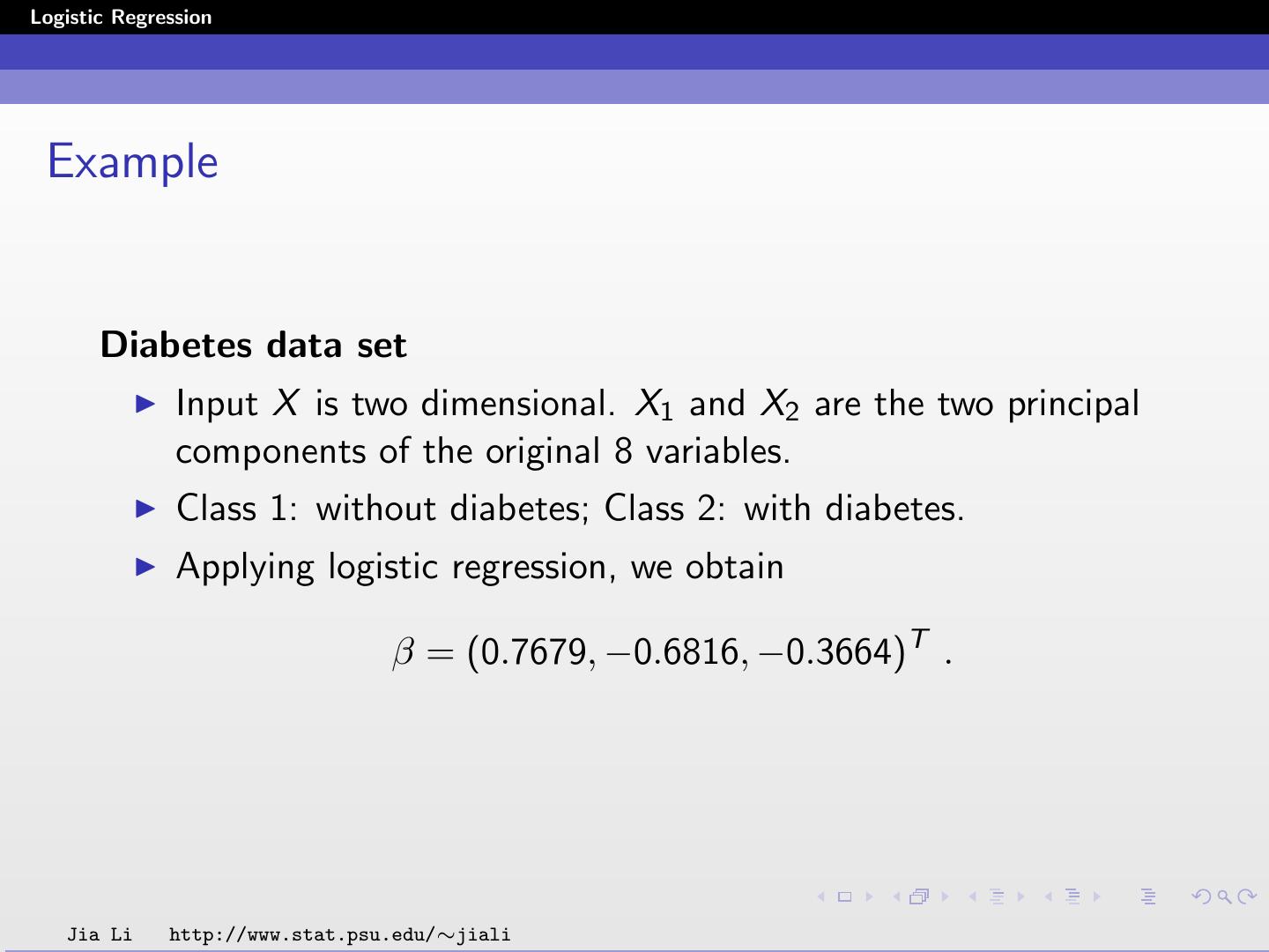
24 .Logistic Regression Example Diabetes data set Input X is two dimensional. X1 and X2 are the two principal components of the original 8 variables. Class 1: without diabetes; Class 2: with diabetes. Applying logistic regression, we obtain β = (0.7679, −0.6816, −0.3664)T . Jia Li http://www.stat.psu.edu/∼jiali 

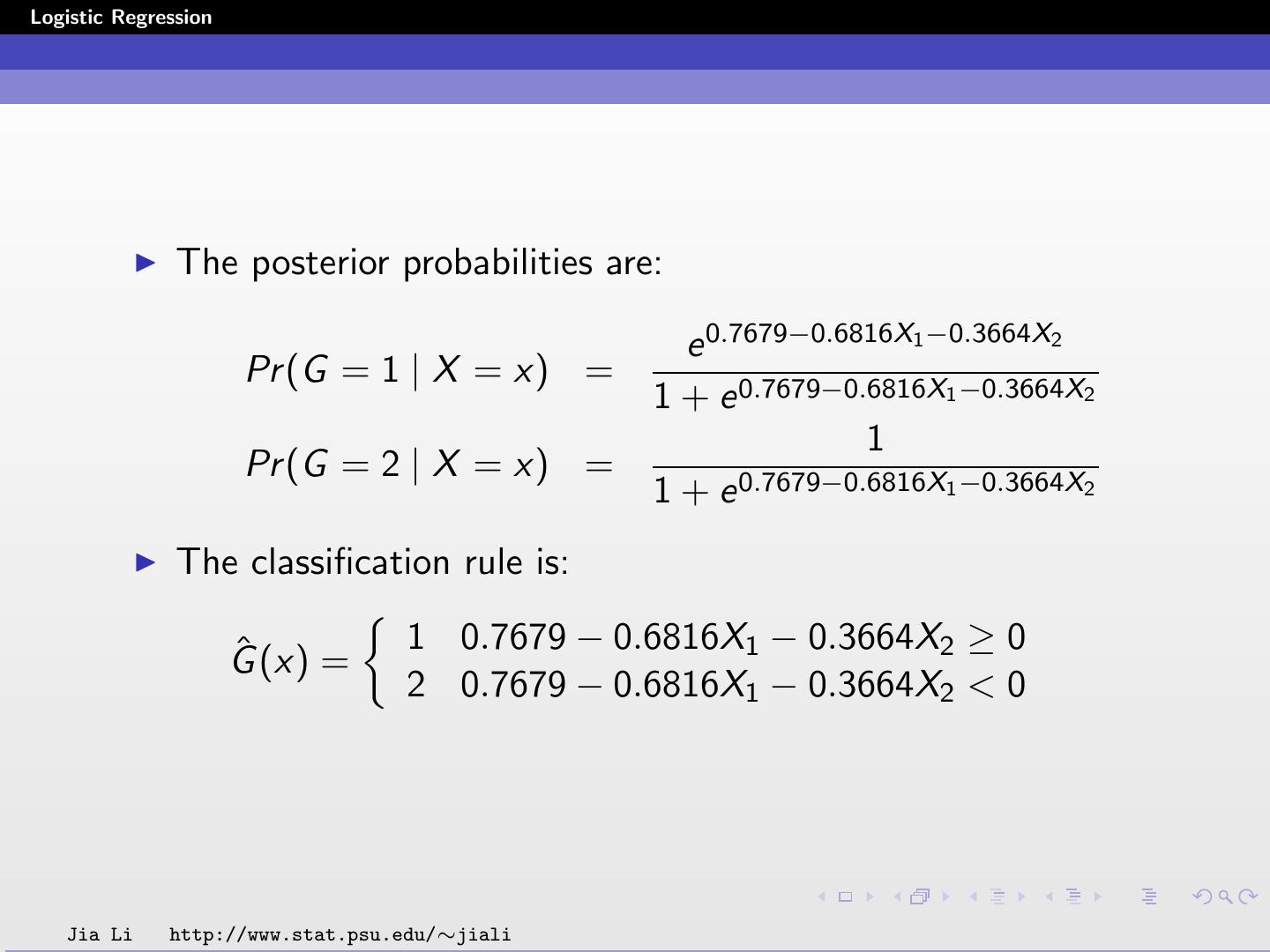
25 .Logistic Regression The posterior probabilities are: e 0.7679−0.6816X1 −0.3664X2 Pr (G = 1 | X = x) = 1 + e 0.7679−0.6816X1 −0.3664X2 1 Pr (G = 2 | X = x) = 1 + e 0.7679−0.6816X1 −0.3664X2 The classification rule is: ˆ (x) = 1 0.7679 − 0.6816X1 − 0.3664X2 ≥ 0 G 2 0.7679 − 0.6816X1 − 0.3664X2 < 0 Jia Li http://www.stat.psu.edu/∼jiali 

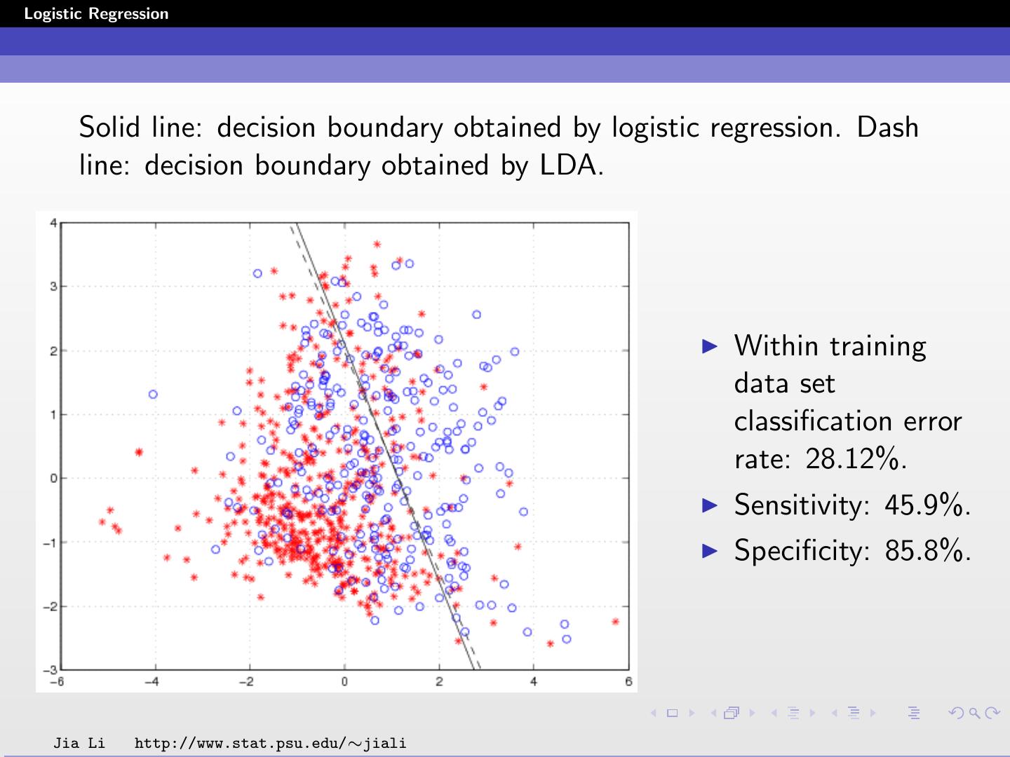
26 .Logistic Regression Solid line: decision boundary obtained by logistic regression. Dash line: decision boundary obtained by LDA. Within training data set classification error rate: 28.12%. Sensitivity: 45.9%. Specificity: 85.8%. Jia Li http://www.stat.psu.edu/∼jiali 

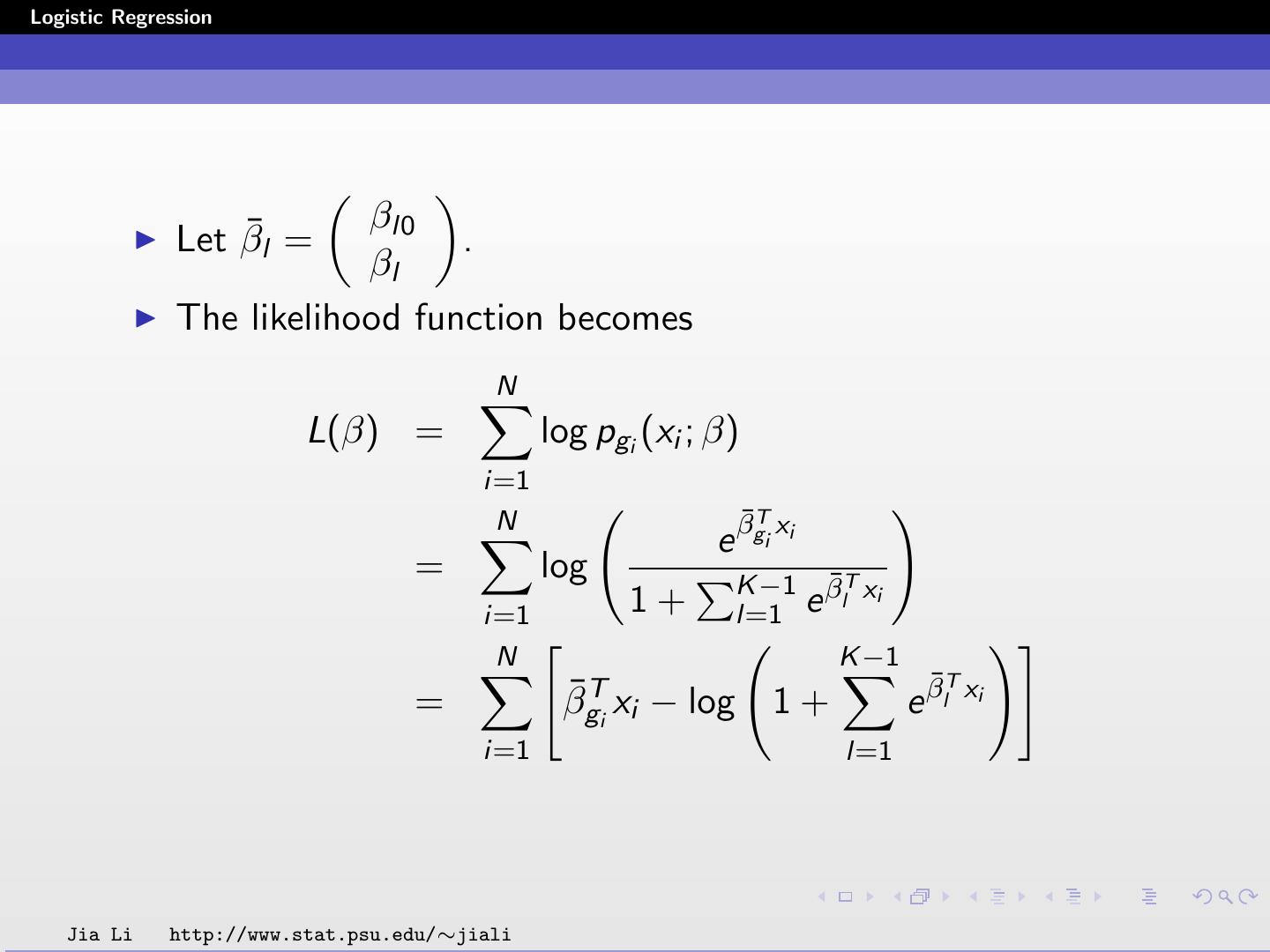
27 .Logistic Regression Multiclass Case (K ≥ 3) When K ≥ 3, β is a (K-1)(p+1)-vector:   β10  β11    .    ..   β10     β1   β1p       β20   β20       .  β2   .  β= = .   ..    β2p    .     .  β(K −1)0    ..   βK −1    β(K −1)0     ..   .  β(K −1)p Jia Li http://www.stat.psu.edu/∼jiali 

28 .Logistic Regression βl0 Let β¯l = . βl The likelihood function becomes N L(β) = log pgi (xi ; β) i=1 N ¯T e βgi xi = log K −1 β¯lT xi i=1 1+ l=1 e N K −1 ¯T xi = β¯gTi xi − log 1 + e βl i=1 l=1 Jia Li http://www.stat.psu.edu/∼jiali 

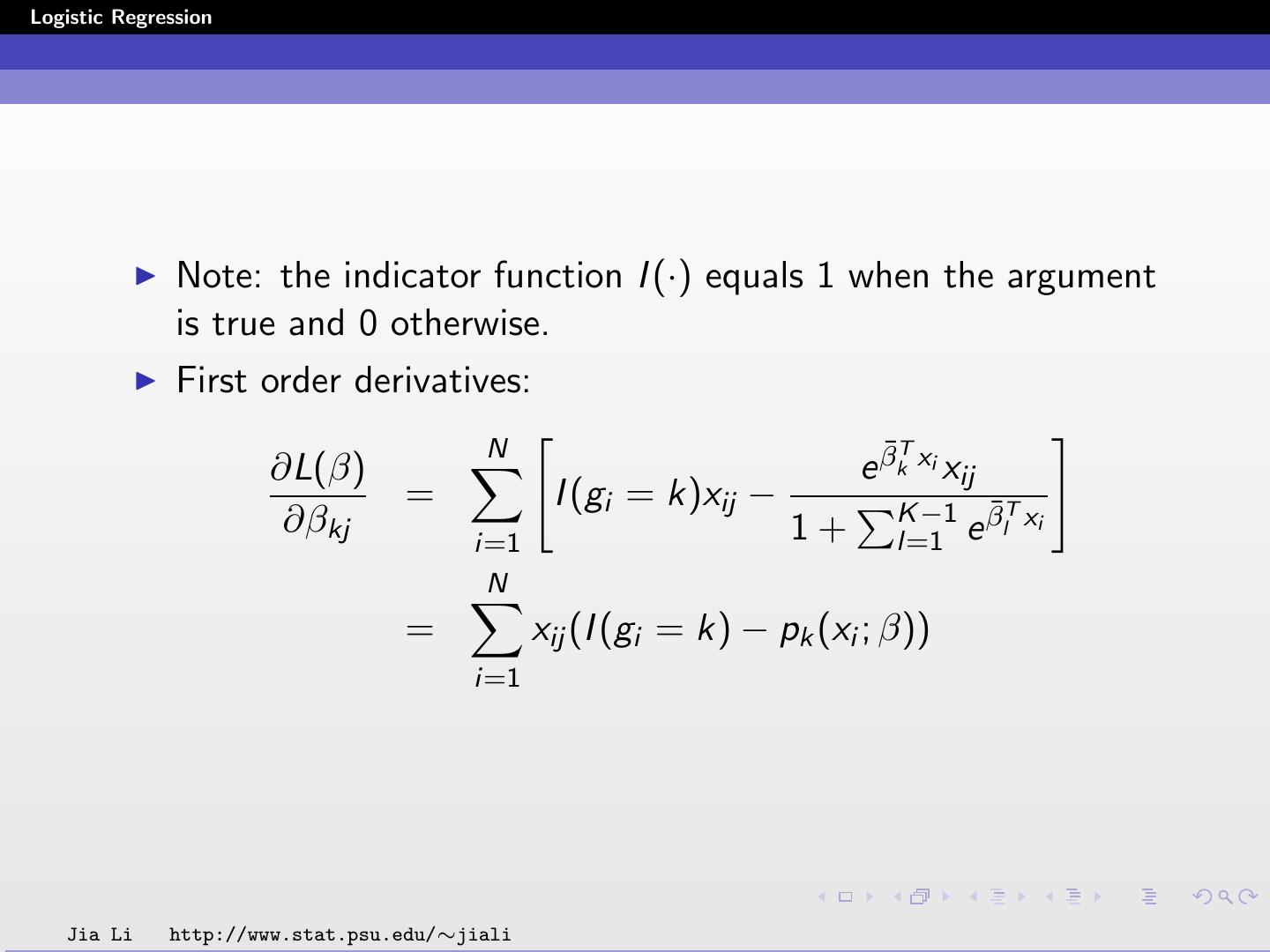
29 .Logistic Regression Note: the indicator function I (·) equals 1 when the argument is true and 0 otherwise. First order derivatives: N ¯T ∂L(β) e βk xi xij = I (gi = k)xij − K −1 β¯lT xi ∂βkj 1+ l=1 e i=1 N = xij (I (gi = k) − pk (xi ; β)) i=1 Jia Li http://www.stat.psu.edu/∼jiali