1 .Computer vision: models, learning and inference Chapter 2 Introduction to probability

2 .Random variables A random variable x denotes a quantity that is uncertain May be result of experiment (flipping a coin) or a real world measurements (measuring temperature) Observing more instances of x, we get different values Some values occur more than others and this information is captured by a probability distribution 2 Computer vision: models, learning and inference. ©2011 Simon J.D. Prince

3 .Discrete Random Variables 3 Computer vision: models, learning and inference. ©2011 Simon J.D. Prince Photo by DaylandS

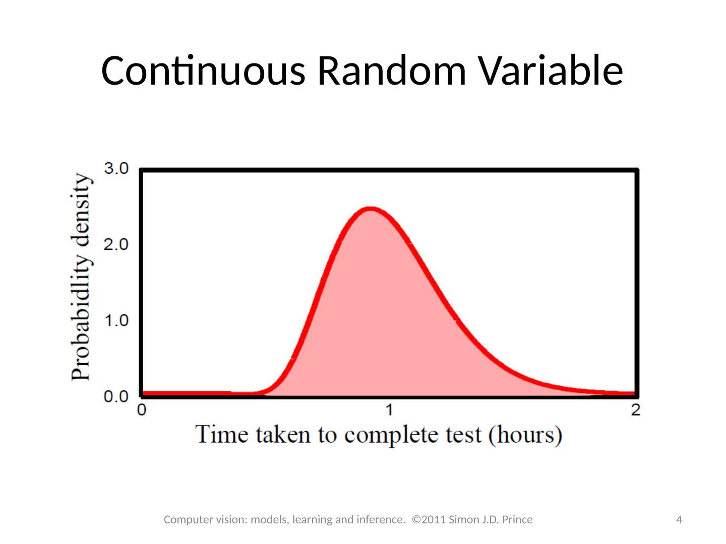
4 .Continuous Random Variable 4 Computer vision: models, learning and inference. ©2011 Simon J.D. Prince

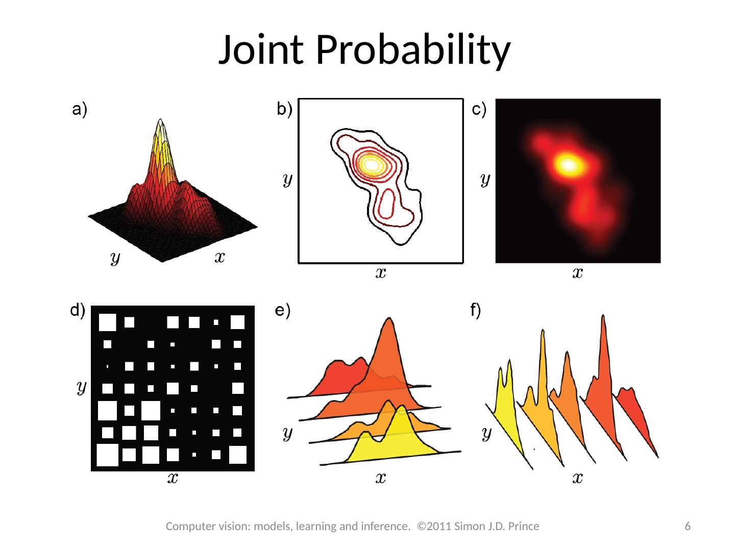
5 .Joint Probability Consider two random variables x and y If we observe multiple paired instances, then some combinations of outcomes are more likely than others This is captured in the joint probability distribution Written as Pr( x , y ) Can read Pr( x , y ) as “probability of x and y ” 5 Computer vision: models, learning and inference. ©2011 Simon J.D. Prince

6 .Joint Probability 6 Computer vision: models, learning and inference. ©2011 Simon J.D. Prince

7 .Marginalization We can recover the probability distribution of any variable in a joint distribution by integrating (or summing) over the other variables 7 Computer vision: models, learning and inference. ©2011 Simon J.D. Prince

8 .Marginalization We can recover the probability distribution of any variable in a joint distribution by integrating (or summing) over the other variables 8 Computer vision: models, learning and inference. ©2011 Simon J.D. Prince

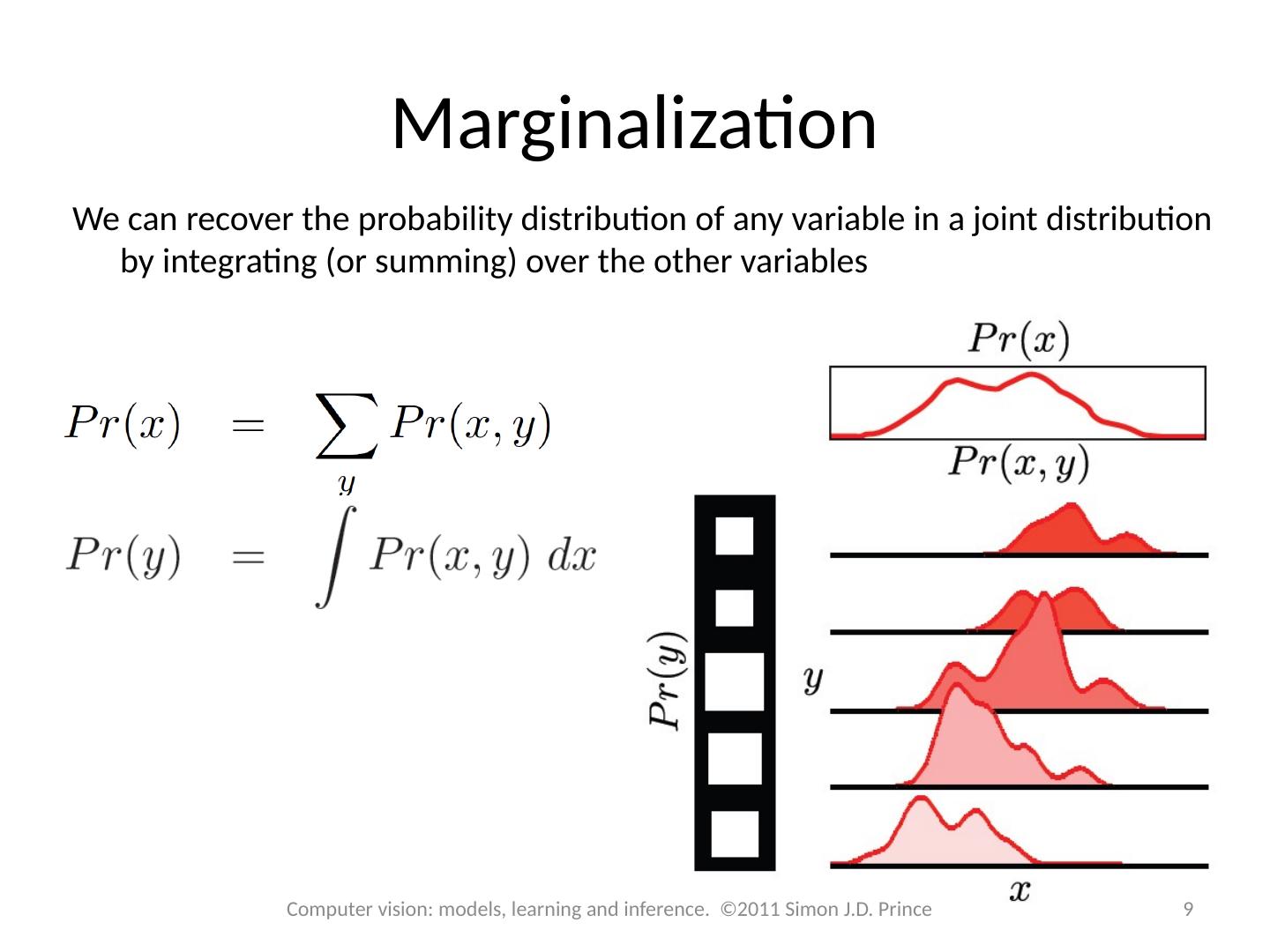
9 .Marginalization We can recover the probability distribution of any variable in a joint distribution by integrating (or summing) over the other variables 9 Computer vision: models, learning and inference. ©2011 Simon J.D. Prince

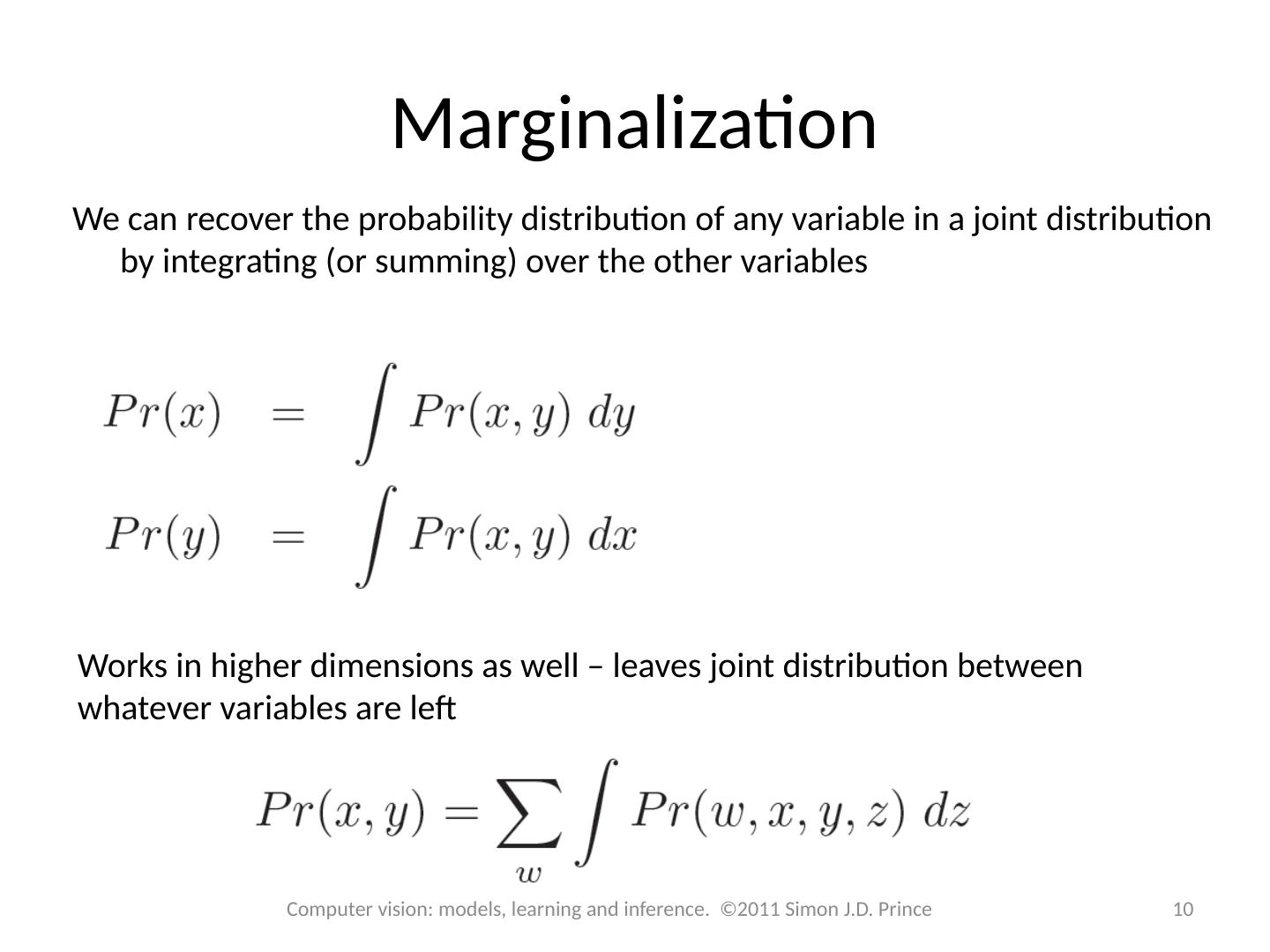
10 .Marginalization We can recover the probability distribution of any variable in a joint distribution by integrating (or summing) over the other variables Works in higher dimensions as well – leaves joint distribution between whatever variables are left 10 Computer vision: models, learning and inference. ©2011 Simon J.D. Prince

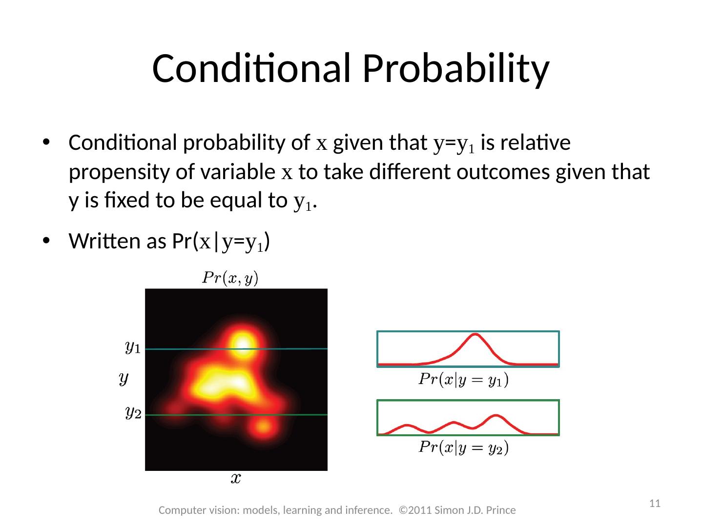
11 .Conditional Probability Conditional probability of x given that y = y 1 is relative propensity of variable x to take different outcomes given that y is fixed to be equal to y 1 . Written as Pr( x | y = y 1 ) 11 Computer vision: models, learning and inference. ©2011 Simon J.D. Prince

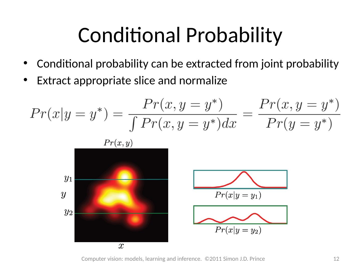
12 .Conditional Probability Conditional probability can be extracted from joint probability Extract appropriate slice and normalize 12 Computer vision: models, learning and inference. ©2011 Simon J.D. Prince

13 .Conditional Probability More usually written in compact form Can be re-arranged to give 13 Computer vision: models, learning and inference. ©2011 Simon J.D. Prince

14 .Conditional Probability This idea can be extended to more than two variables 14 Computer vision: models, learning and inference. ©2011 Simon J.D. Prince

15 .Bayes ’ Rule From before: Combining: Re-arranging: 15 Computer vision: models, learning and inference. ©2011 Simon J.D. Prince

16 .Bayes ’ Rule Terminology Posterior – what we know about y after seeing x 16 Computer vision: models, learning and inference. ©2011 Simon J.D. Prince Prior – what we know about y before seeing x Likelihood – propensity for observing a certain value of x given a certain value of y Evidence –a constant to ensure that the left hand side is a valid distribution

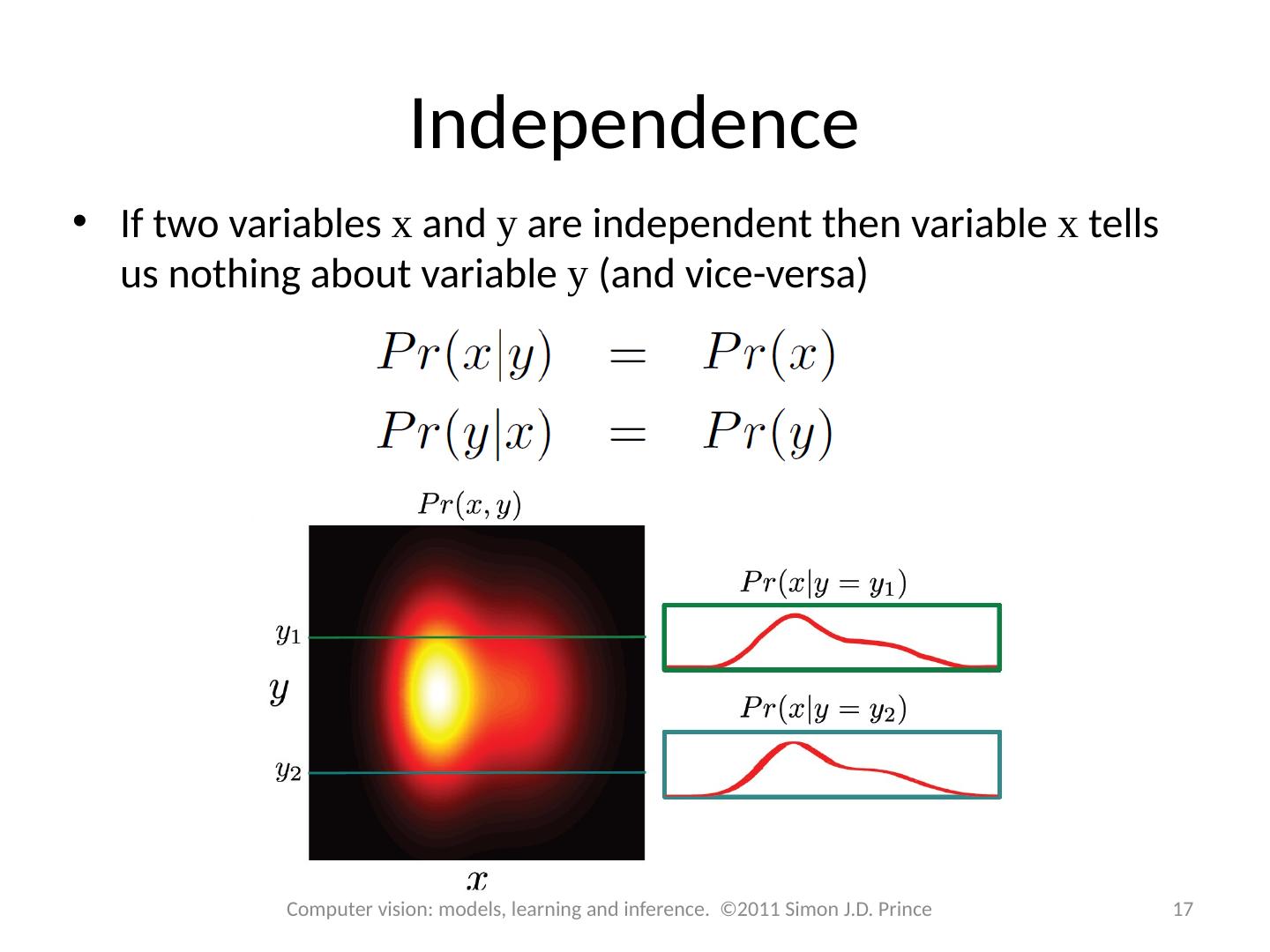
17 .Independence If two variables x and y are independent then variable x tells us nothing about variable y (and vice-versa) 17 Computer vision: models, learning and inference. ©2011 Simon J.D. Prince

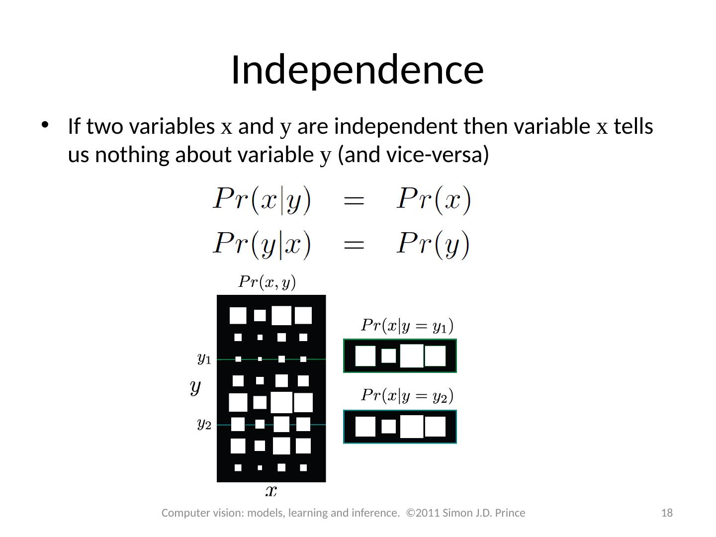
18 .Independence If two variables x and y are independent then variable x tells us nothing about variable y (and vice-versa) 18 Computer vision: models, learning and inference. ©2011 Simon J.D. Prince

19 .Independence When variables are independent, the joint factorizes into a product of the marginals : 19 Computer vision: models, learning and inference. ©2011 Simon J.D. Prince

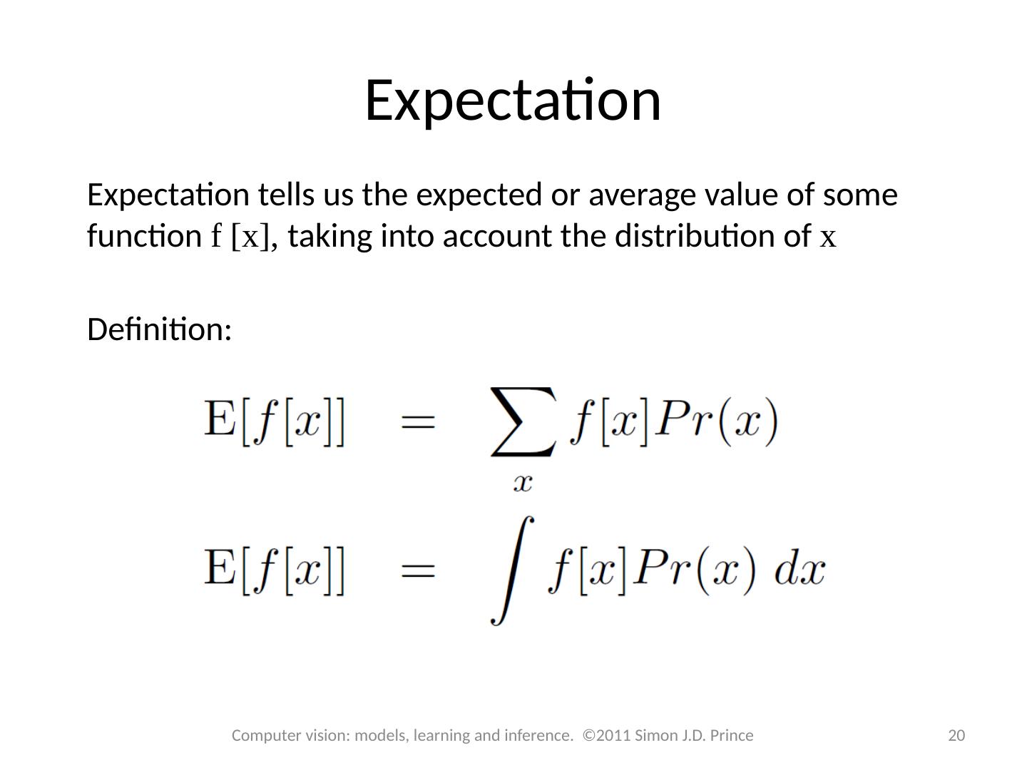
20 .Expectation Expectation tells us the expected or average value of some function f [x], taking into account the distribution of x Definition: 20 Computer vision: models, learning and inference. ©2011 Simon J.D. Prince

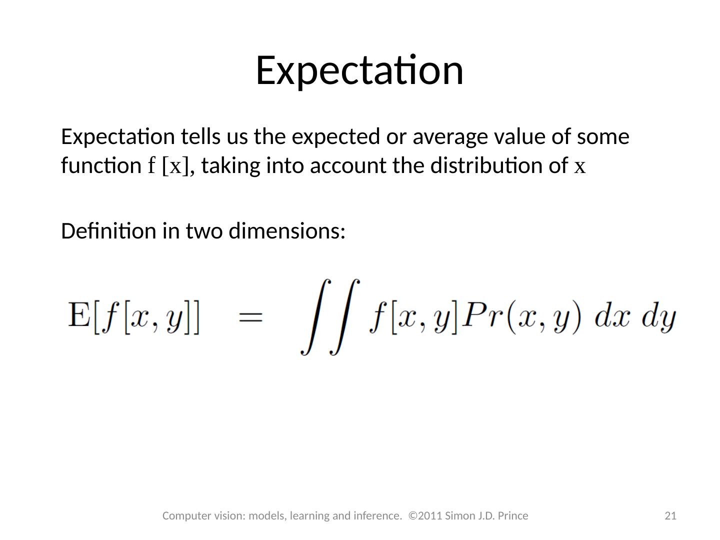
21 .Expectation Expectation tells us the expected or average value of some function f [x], taking into account the distribution of x Definition in two dimensions: 21 Computer vision: models, learning and inference. ©2011 Simon J.D. Prince

22 .Expectation: Common Cases 22 Computer vision: models, learning and inference. ©2011 Simon J.D. Prince

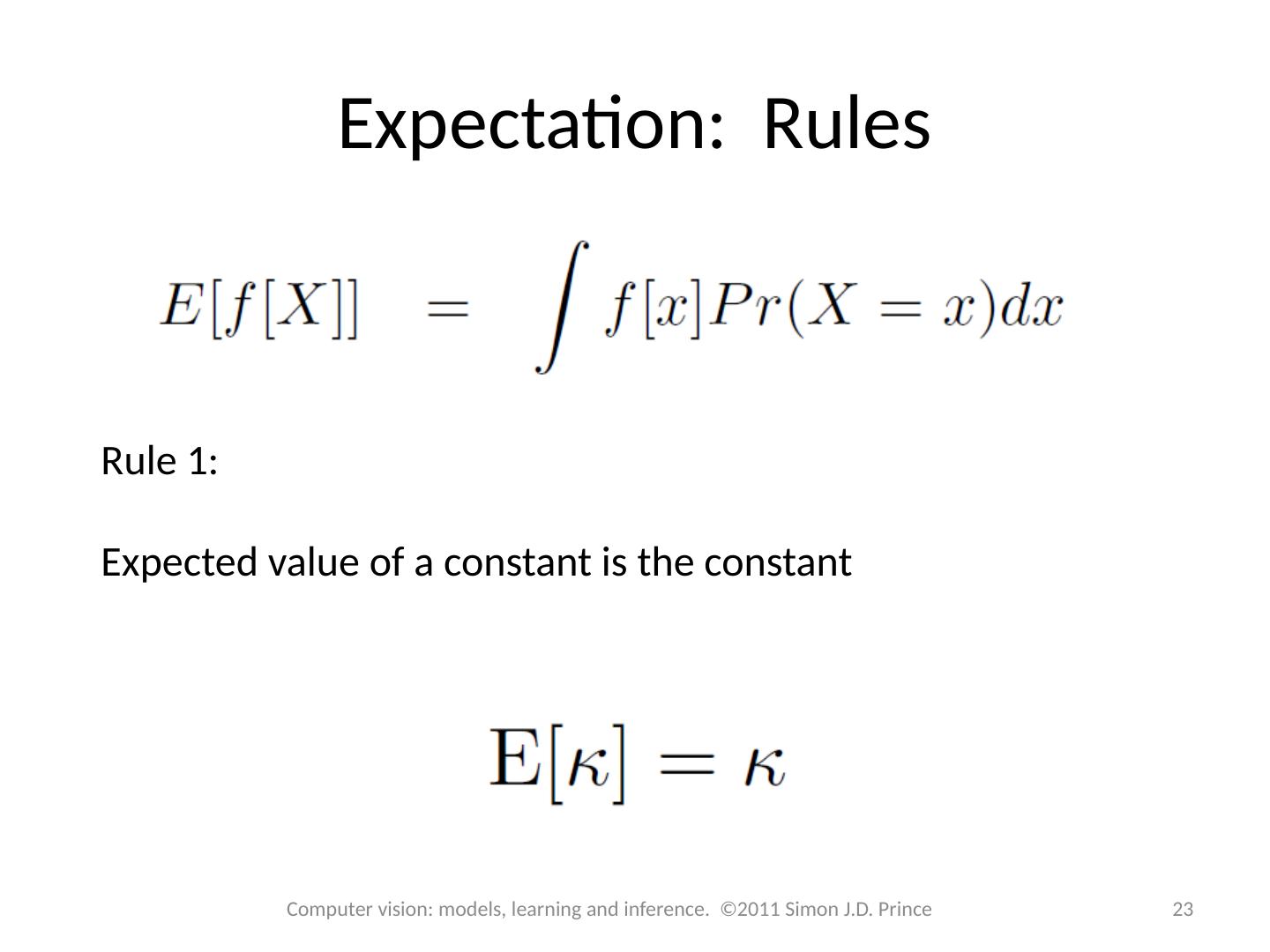
23 .Expectation: Rules Rule 1: Expected value of a constant is the constant 23 Computer vision: models, learning and inference. ©2011 Simon J.D. Prince

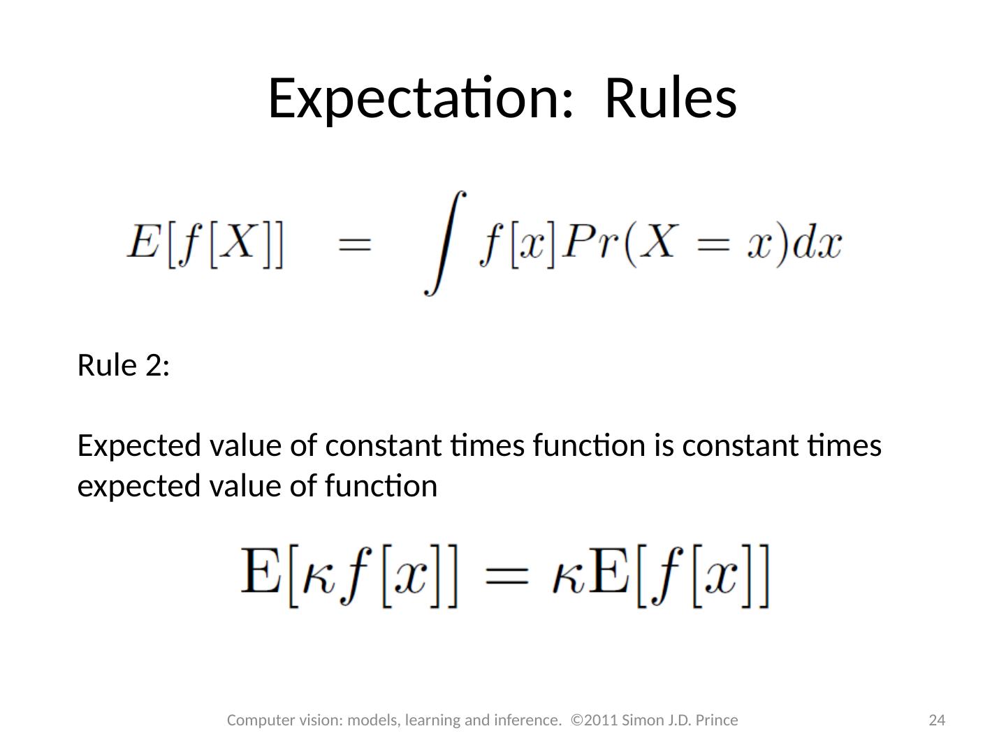
24 .Expectation: Rules Rule 2: Expected value of constant times function is constant times expected value of function 24 Computer vision: models, learning and inference. ©2011 Simon J.D. Prince

25 .Expectation: Rules Rule 3: Expectation of sum of functions is sum of expectation of functions 25 Computer vision: models, learning and inference. ©2011 Simon J.D. Prince

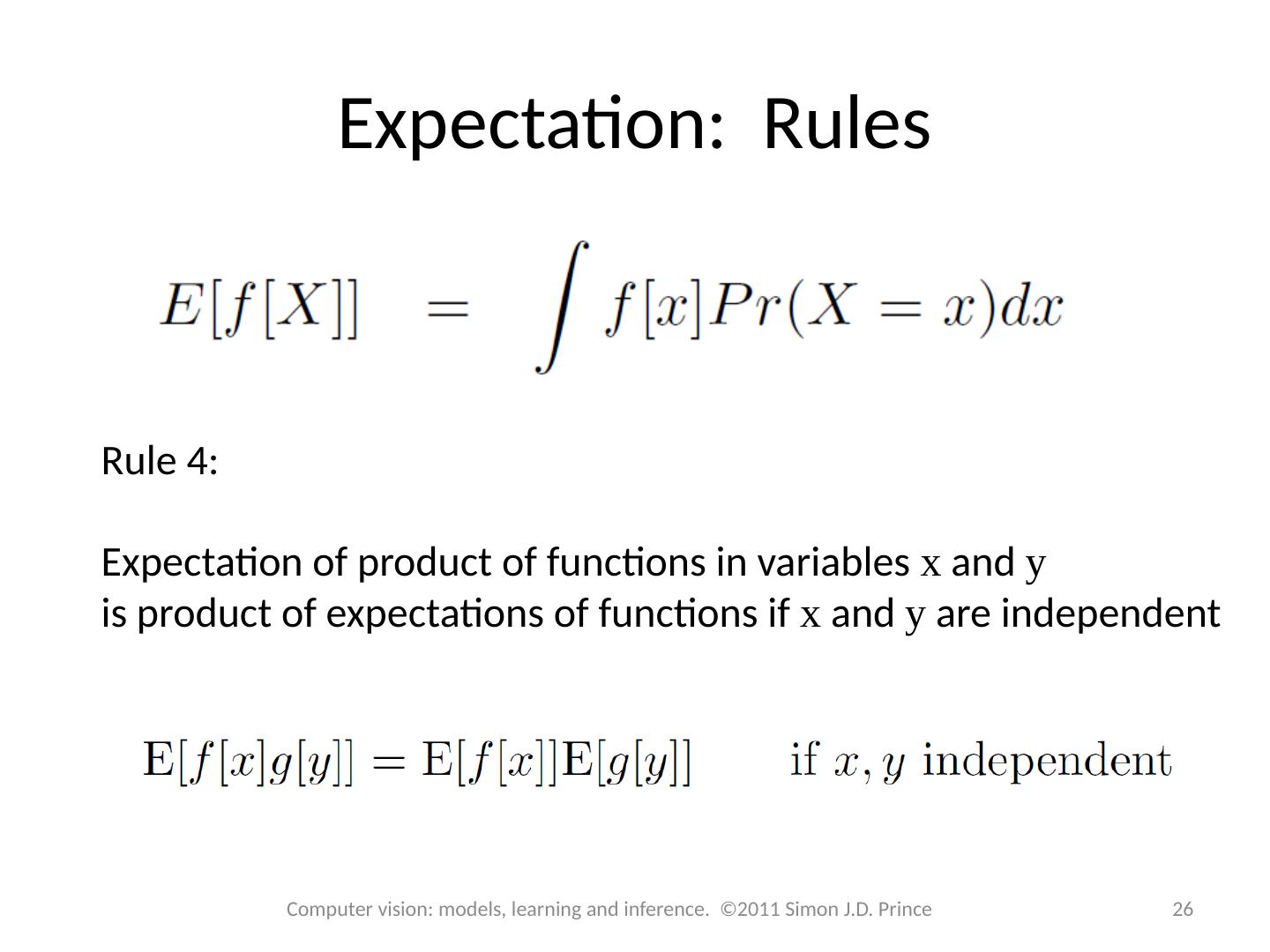
26 .Expectation: Rules Rule 4: Expectation of product of functions in variables x and y is product of expectations of functions if x and y are independent 26 Computer vision: models, learning and inference. ©2011 Simon J.D. Prince

27 .Conclusions 27 Computer vision: models, learning and inference. ©2011 Simon J.D. Prince Rules of probability are compact and simple Concepts of marginalization, joint and conditional probability, Bayes ’ rule and expectation underpin all of the models we use One remaining concept – conditional expectation – discussed later