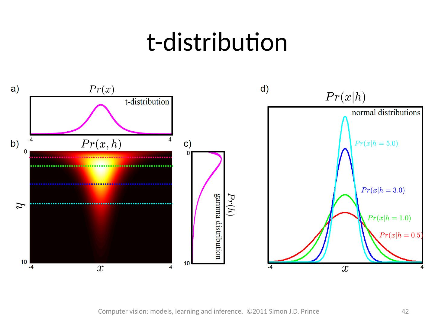
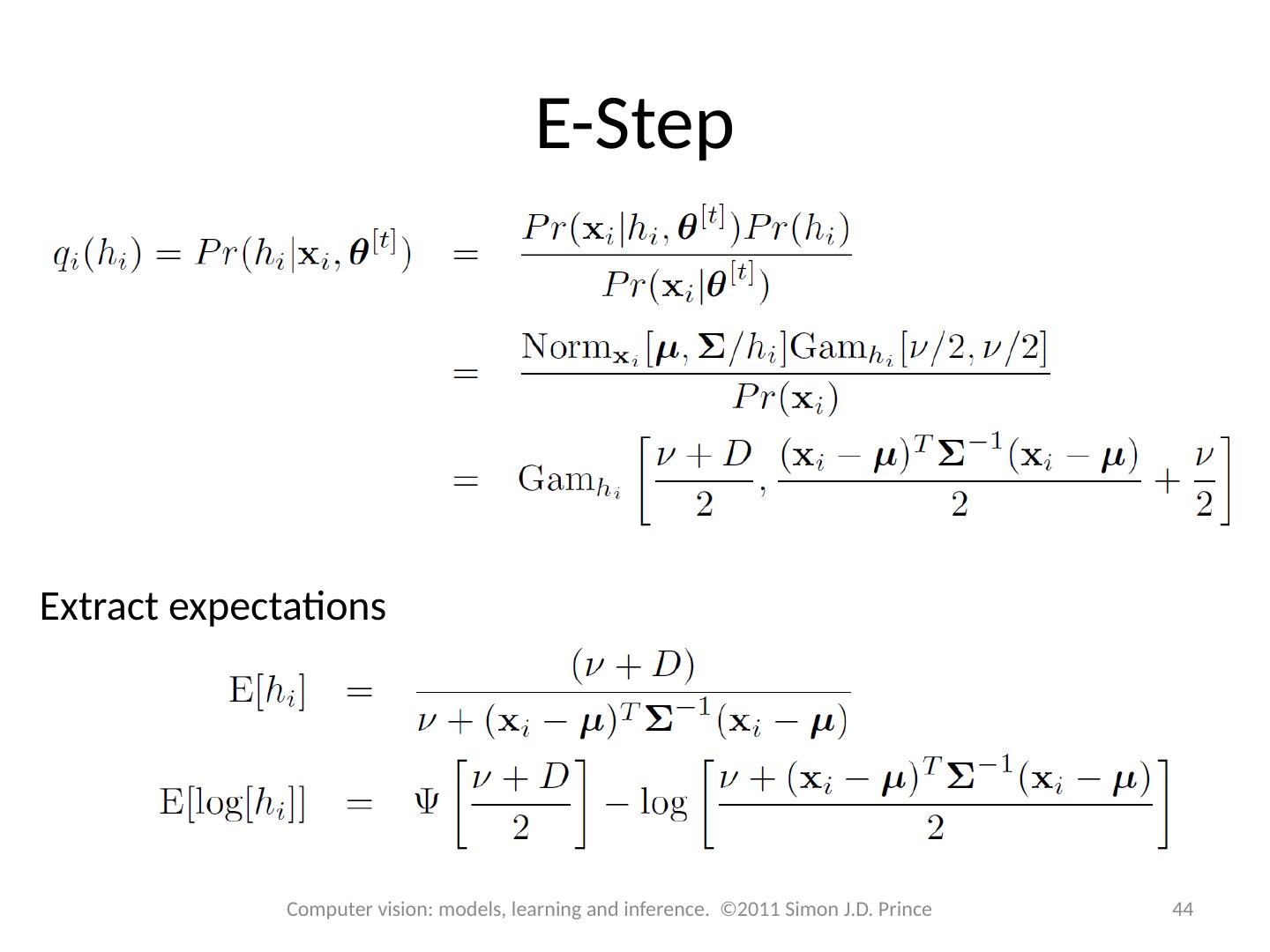
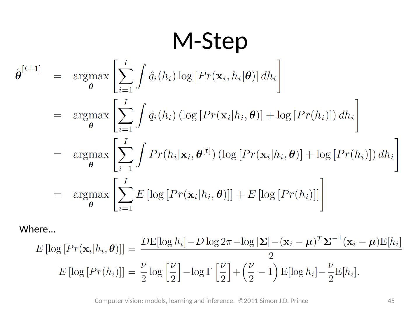
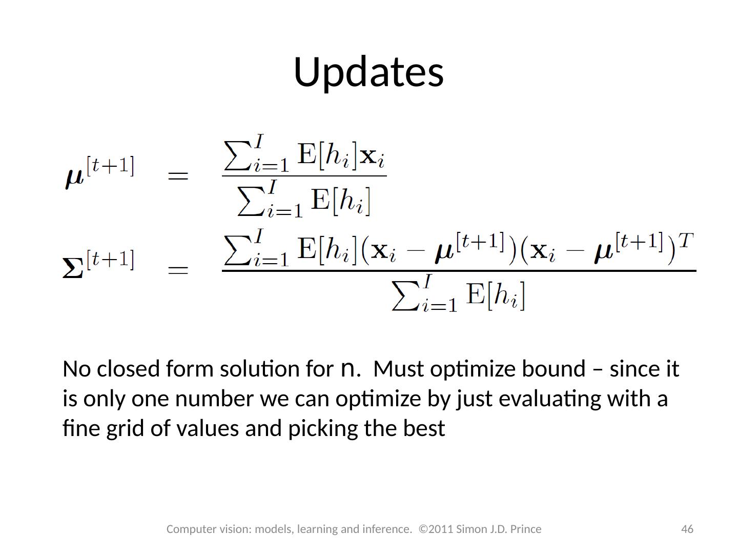
07_Modeling_Complex_Densities

1 .Computer vision: models, learning and inference Chapter 7 Modeling Complex Densities

2 .Structure 2 2 Computer vision: models, learning and inference. ©2011 Simon J.D. Prince Densities for classification Models with hidden variables Mixture of Gaussians t-distributions Factor analysis EM algorithm in detail Applications

3 .Models for machine vision 3 Computer vision: models, learning and inference. ©2011 Simon J.D. Prince

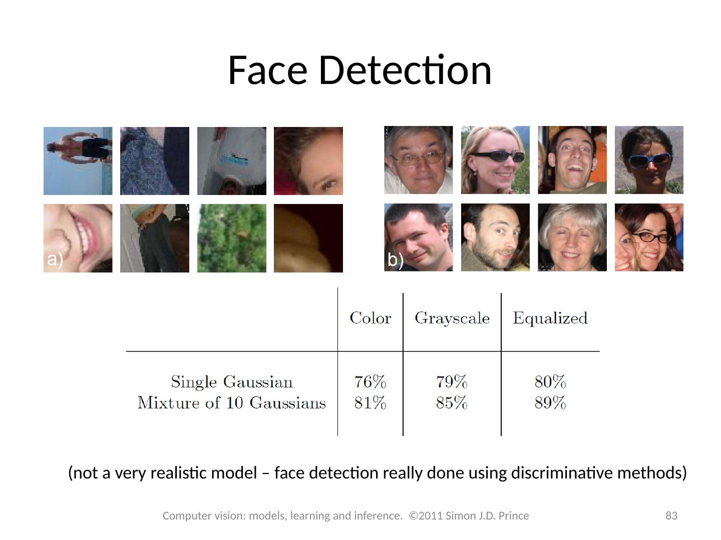
4 .Face Detection 4 Computer vision: models, learning and inference. ©2011 Simon J.D. Prince

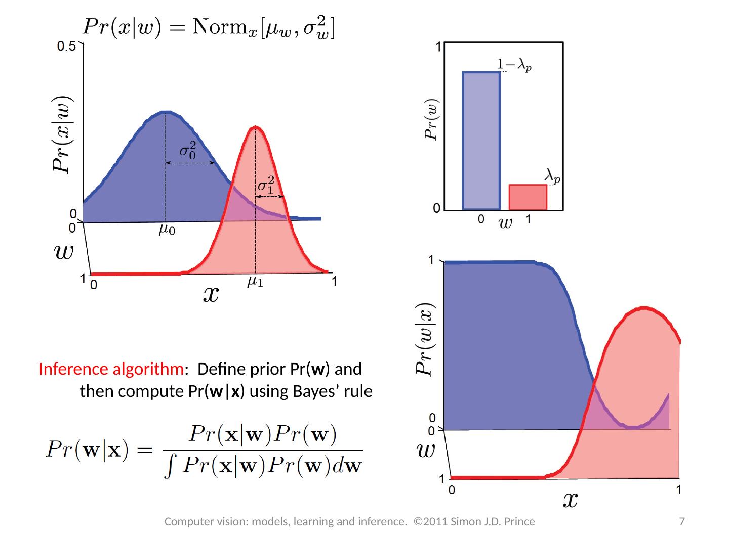
5 .Type 3: Pr( x | w ) - Generative How to model Pr( x | w )? Choose an appropriate form for Pr( x ) Make parameters a function of w Function takes parameters q that define its shape Learning algorithm : learn parameters q from training data x , w Inference algorithm : Define prior Pr( w ) and then compute Pr( w | x ) using Bayes ’ rule 5 Computer vision: models, learning and inference. ©2011 Simon J.D. Prince

6 .Classification Model Or writing in terms of class conditional density functions Parameters m 0 , S 0 learnt just from data S 0 where w=0 Similarly, parameters m 1 , S 1 learnt just from data S 1 where w=1 6 Computer vision: models, learning and inference. ©2011 Simon J.D. Prince

7 .7 Computer vision: models, learning and inference. ©2011 Simon J.D. Prince Inference algorithm : Define prior Pr( w ) and then compute Pr( w | x ) using Bayes ’ rule

8 .Experiment 1000 non-faces 1000 faces 60x60x3 Images =10800 x1 vectors Equal priors Pr(y=1)=Pr(y=0) = 0.5 75% performance on test set. Not very good! 8 Computer vision: models, learning and inference. ©2011 Simon J.D. Prince

9 .Results (diagonal covariance) 9 Computer vision: models, learning and inference. ©2011 Simon J.D. Prince

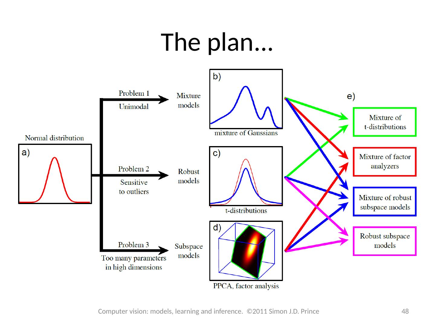
10 .The plan... 10 Computer vision: models, learning and inference. ©2011 Simon J.D. Prince

11 .Structure 11 11 Computer vision: models, learning and inference. ©2011 Simon J.D. Prince Densities for classification Models with hidden variables Mixture of Gaussians t-distributions Factor analysis EM algorithm in detail Applications

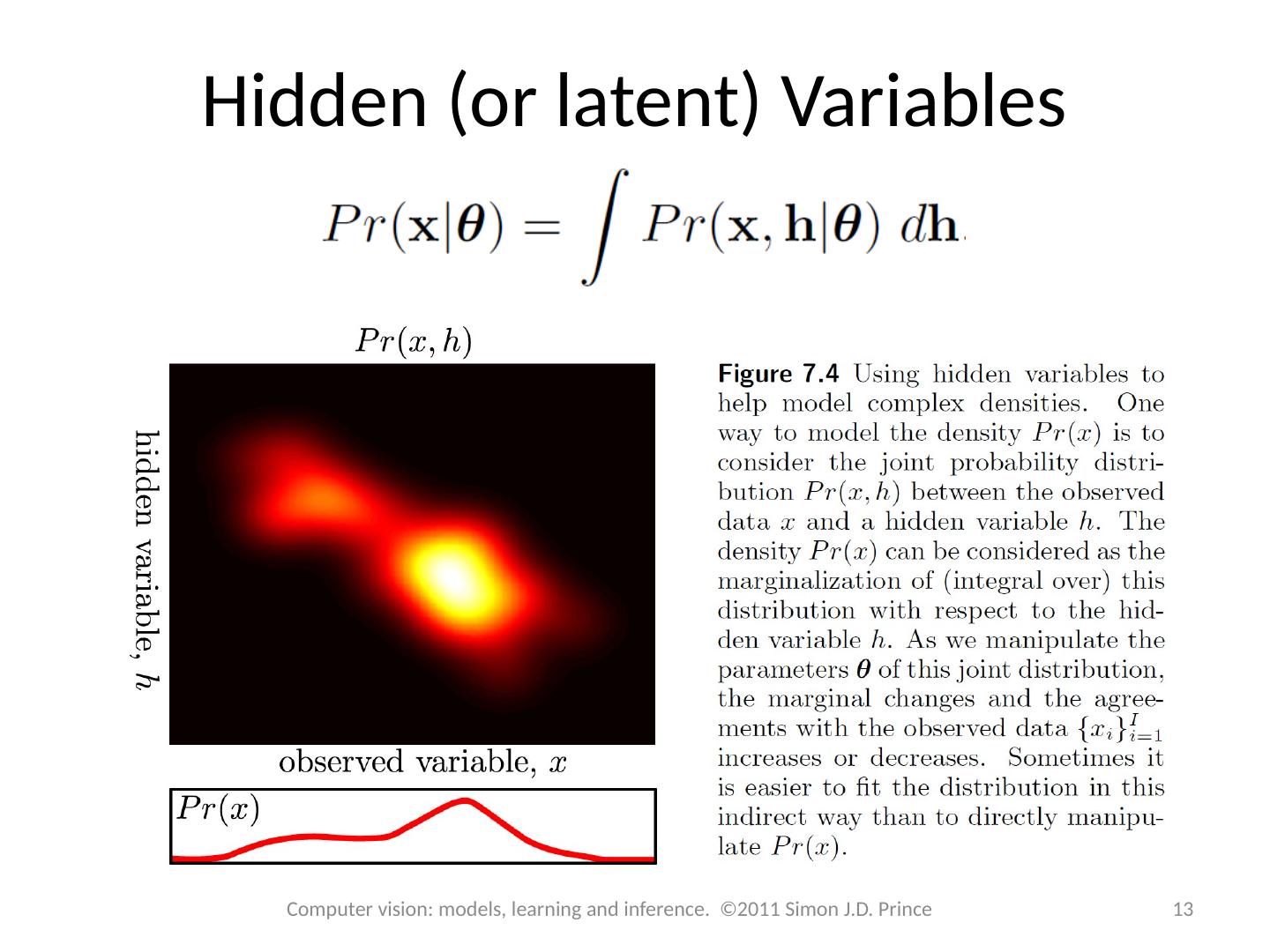
12 .Hidden (or latent) Variables Key idea: represent density Pr(x) as marginalization of joint density with another variable h that we do not see 12 Computer vision: models, learning and inference. ©2011 Simon J.D. Prince Will also depend on some parameters:

13 .Hidden (or latent) Variables 13 Computer vision: models, learning and inference. ©2011 Simon J.D. Prince

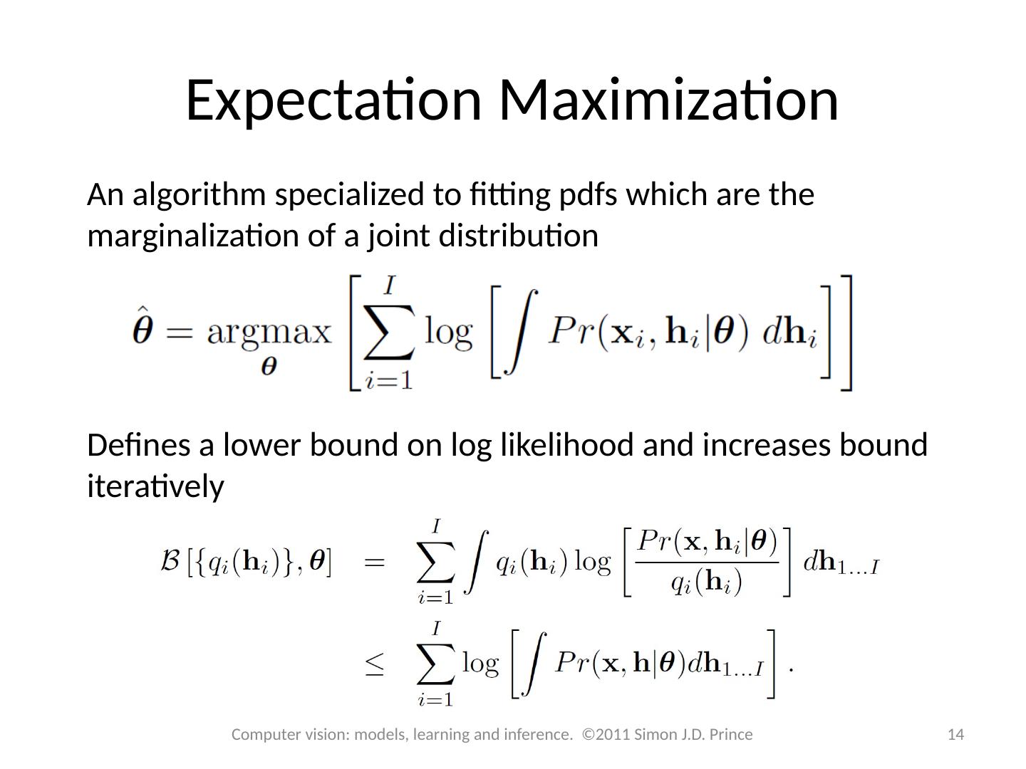
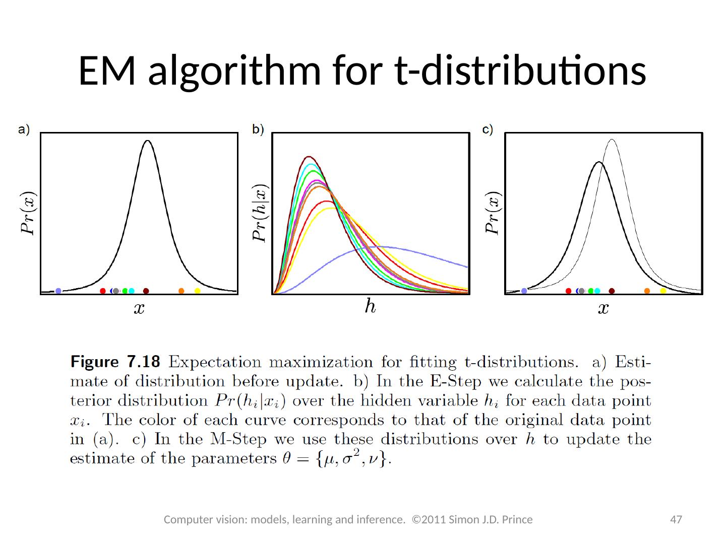
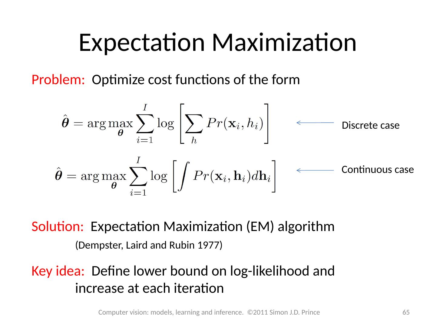
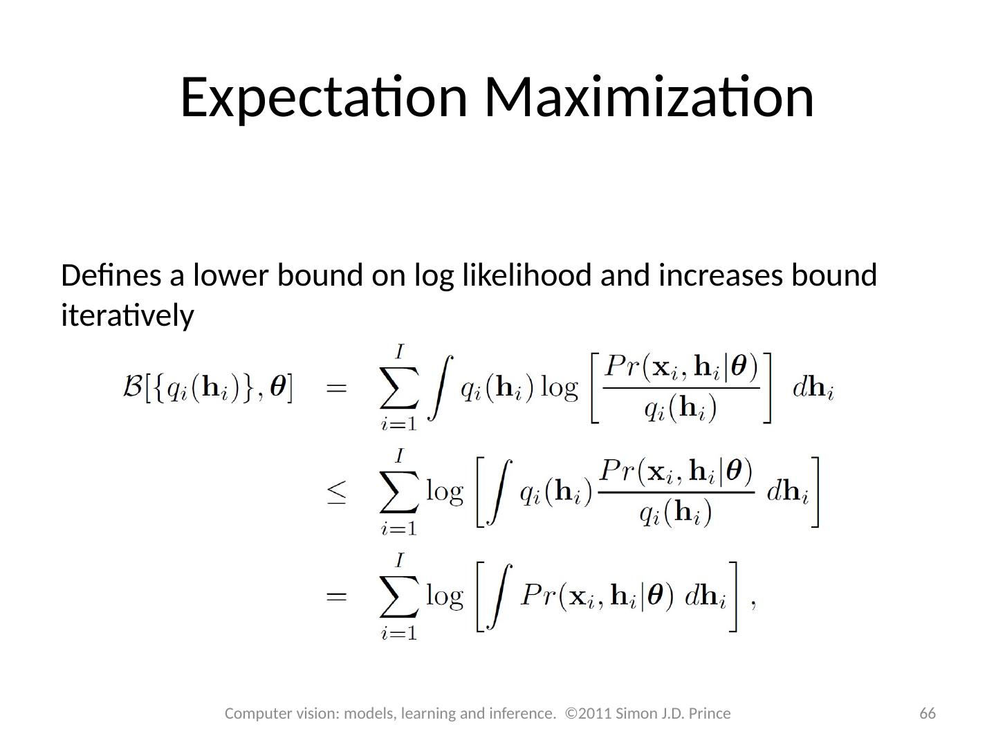
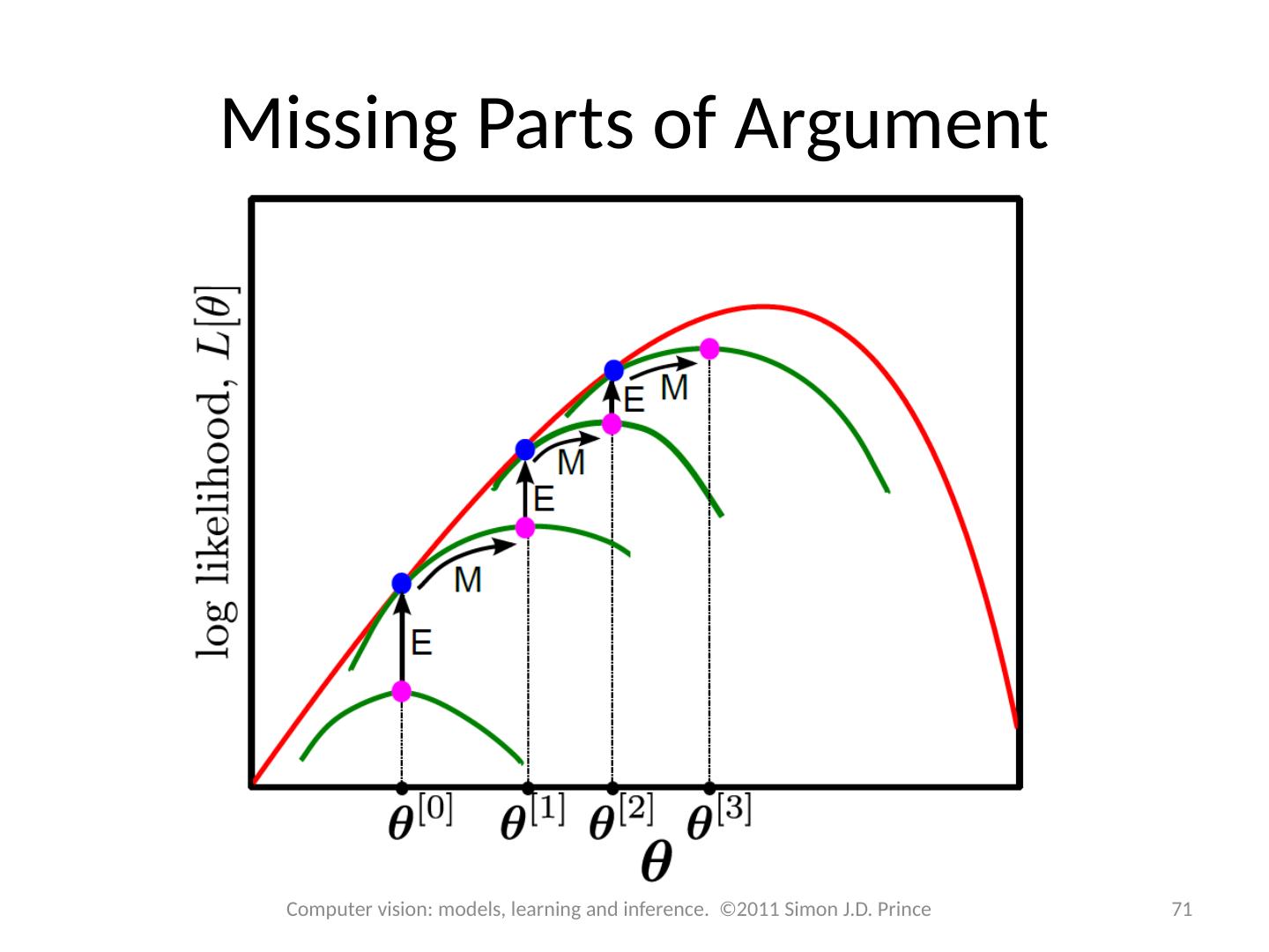
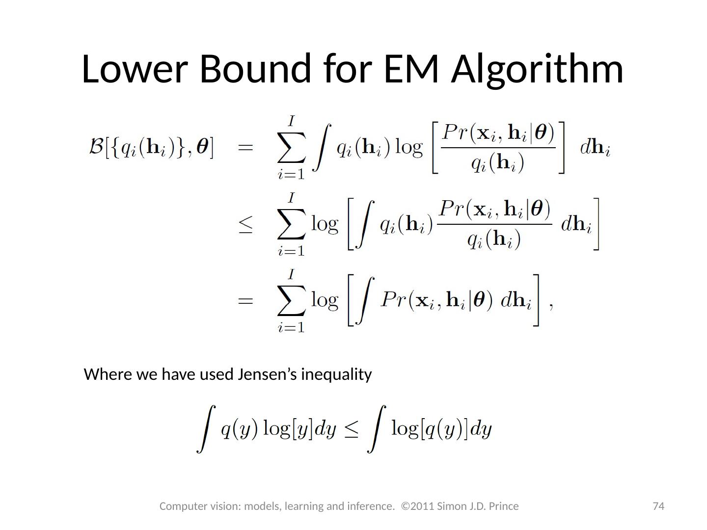
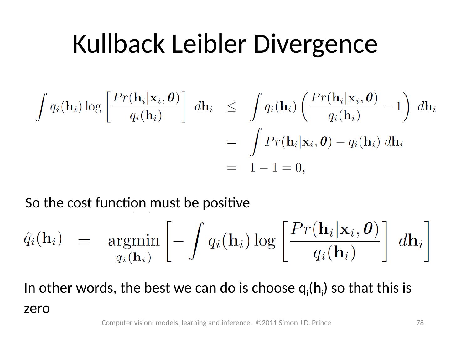
14 .Expectation Maximization An algorithm specialized to fitting pdfs which are the marginalization of a joint distribution Defines a lower bound on log likelihood and increases bound iteratively 14 Computer vision: models, learning and inference. ©2011 Simon J.D. Prince

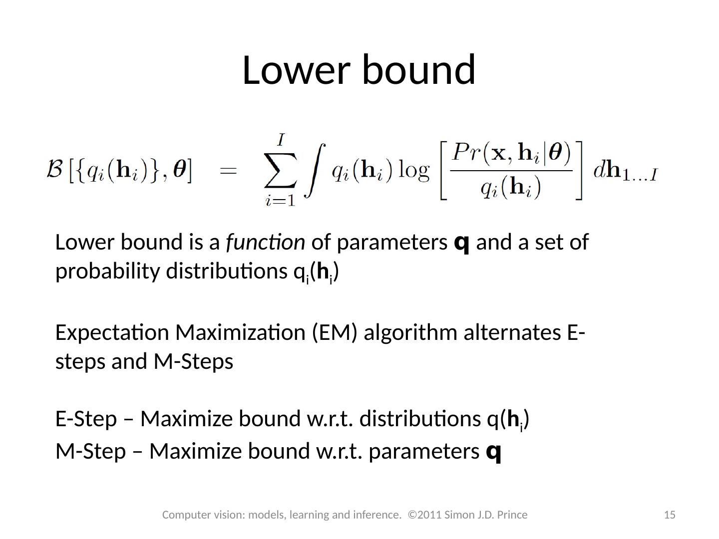
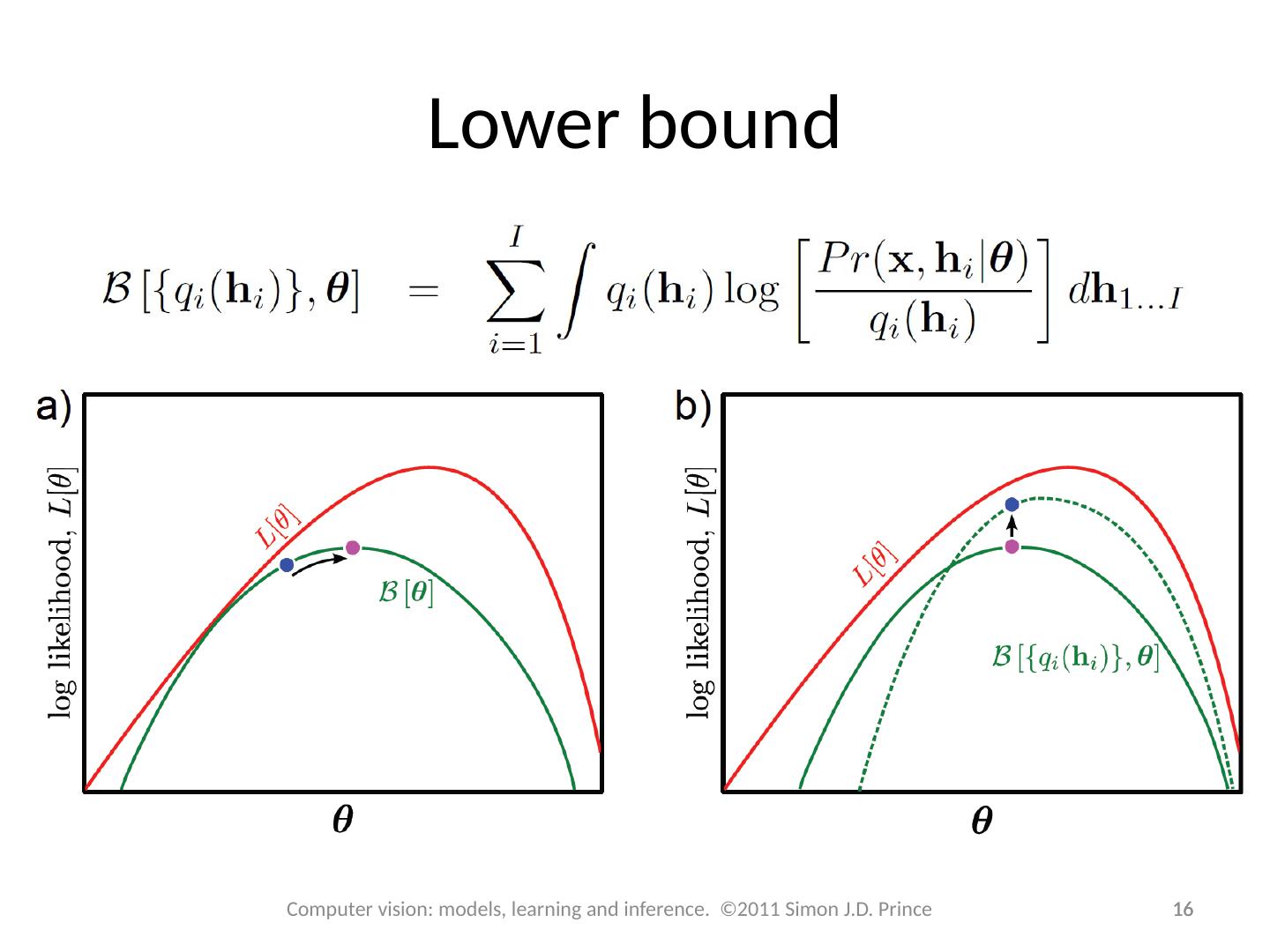
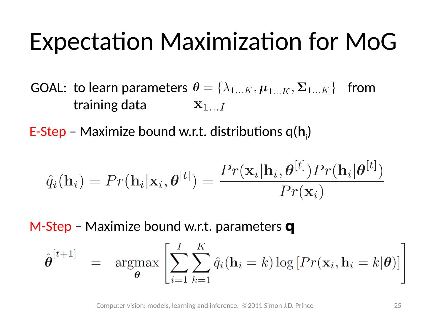
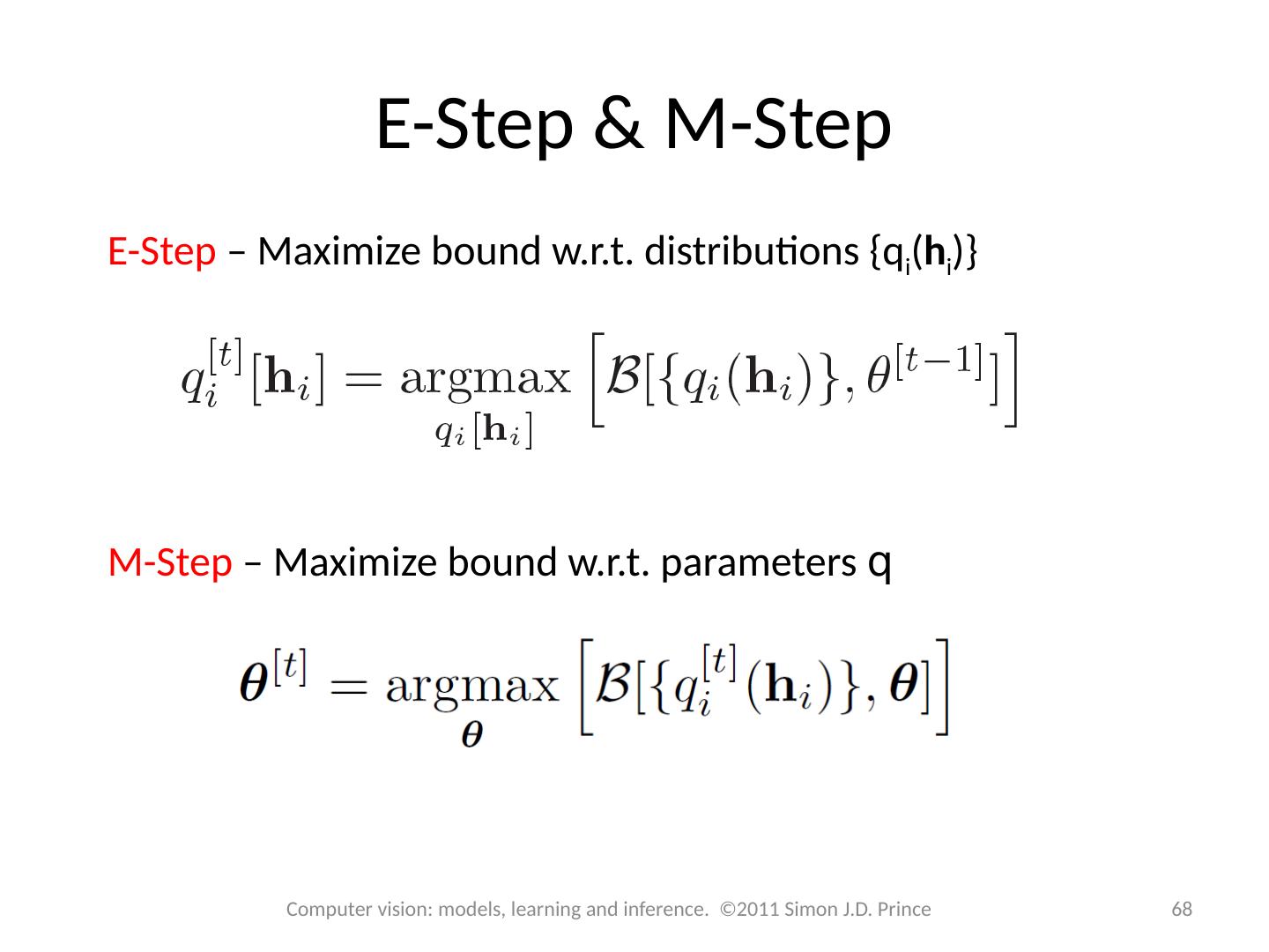
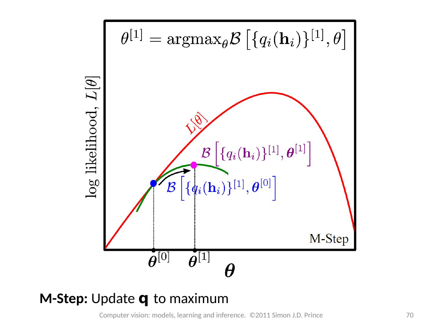
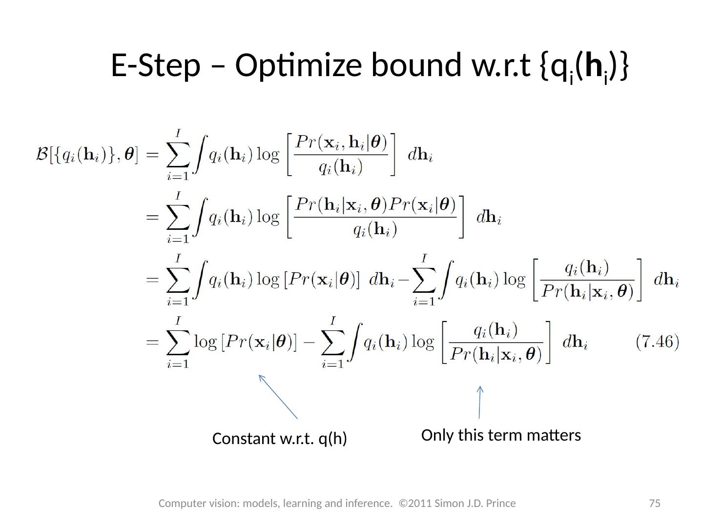
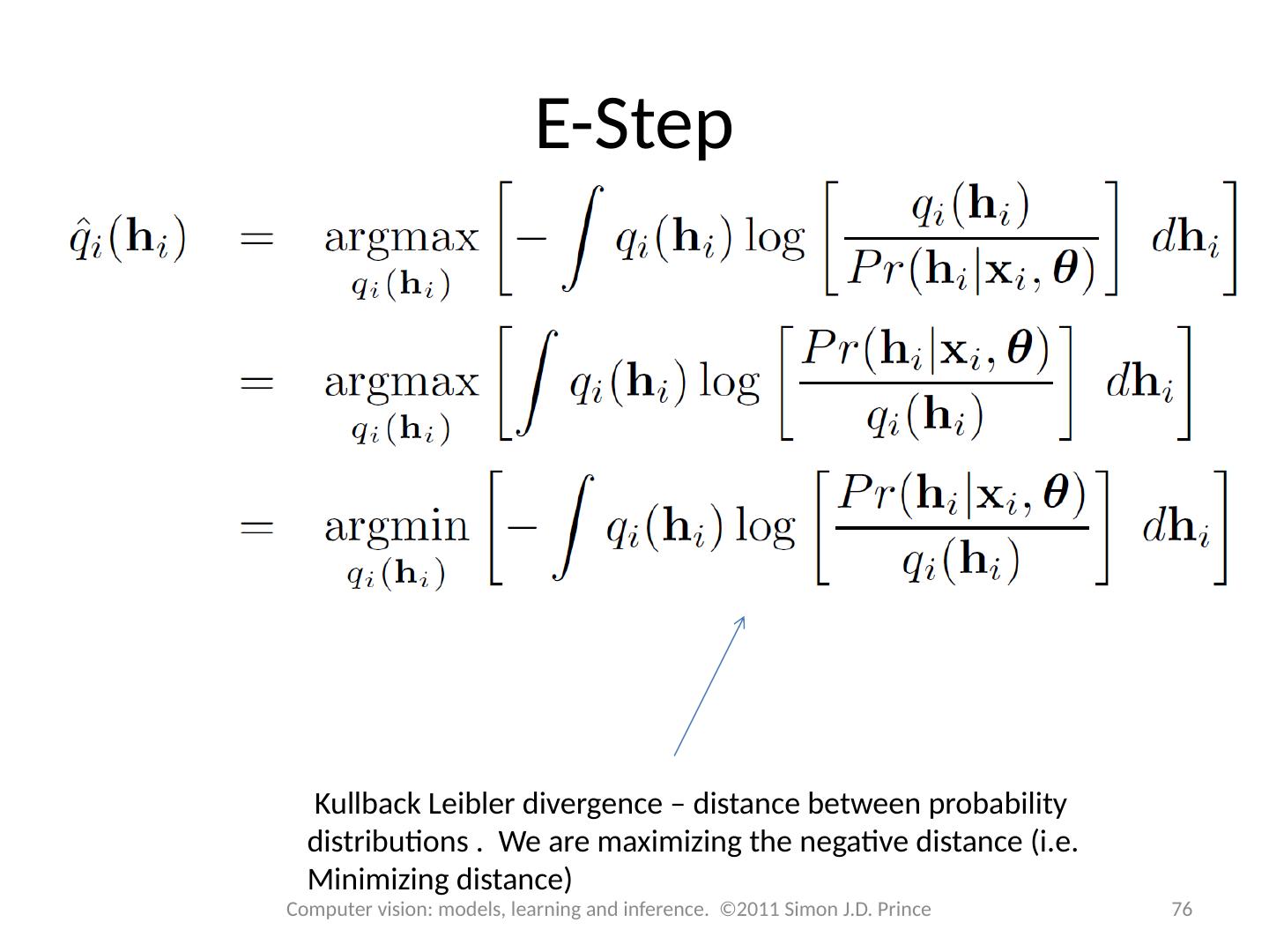
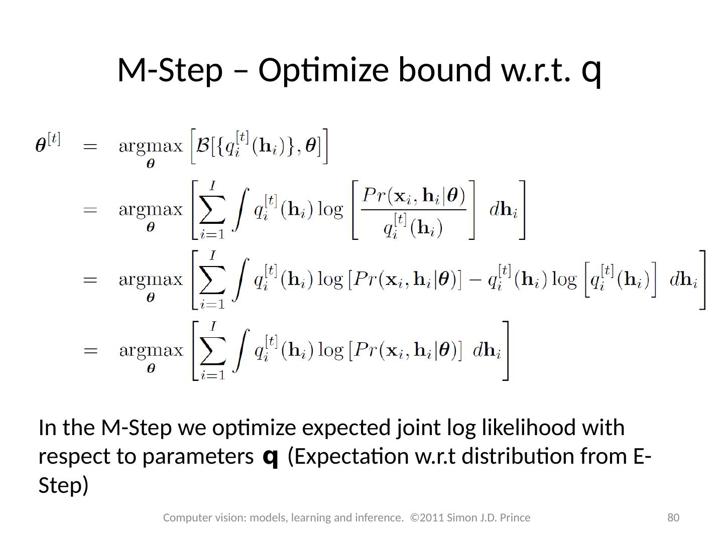
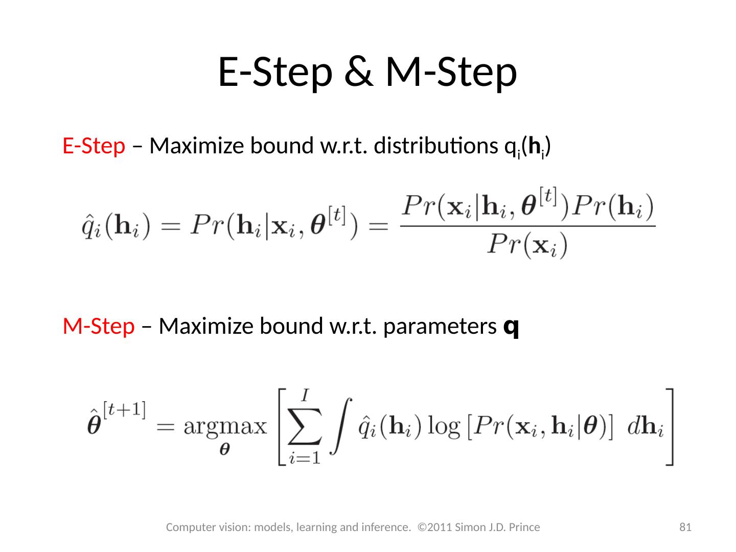
15 .Lower bound Lower bound is a function of parameters q and a set of probability distributions q i ( h i ) Expectation Maximization (EM) algorithm alternates E-steps and M-Steps E-Step – Maximize bound w.r.t . distributions q( h i ) M-Step – Maximize bound w.r.t . parameters q 15 Computer vision: models, learning and inference. ©2011 Simon J.D. Prince

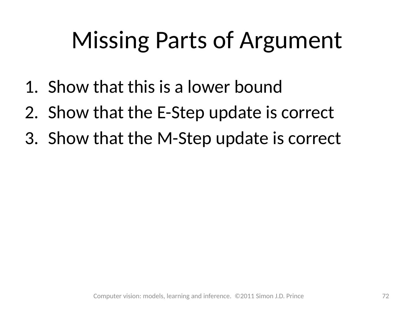
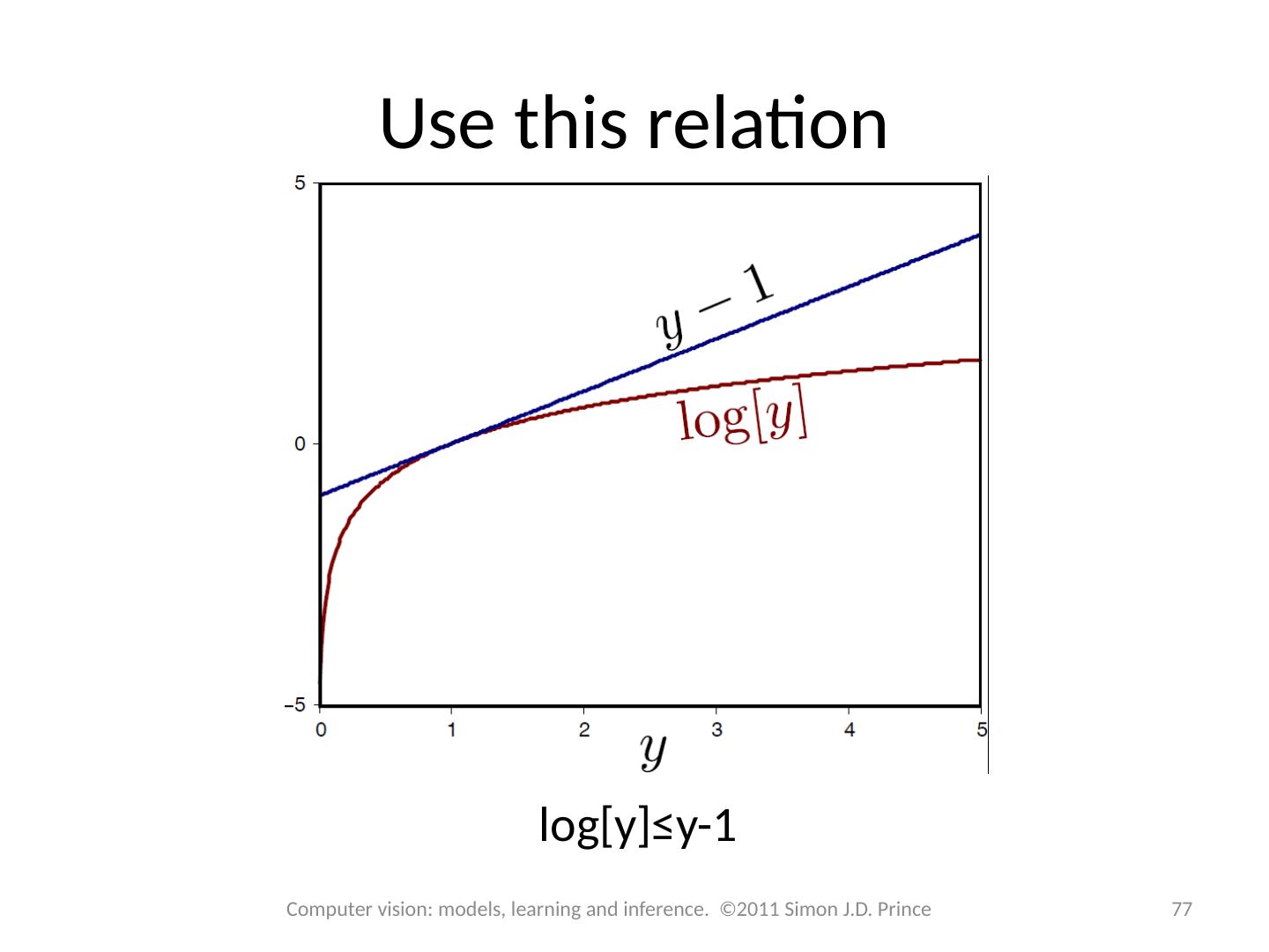
16 .Computer vision: models, learning and inference. ©2011 Simon J.D. Prince 16 Lower bound 16

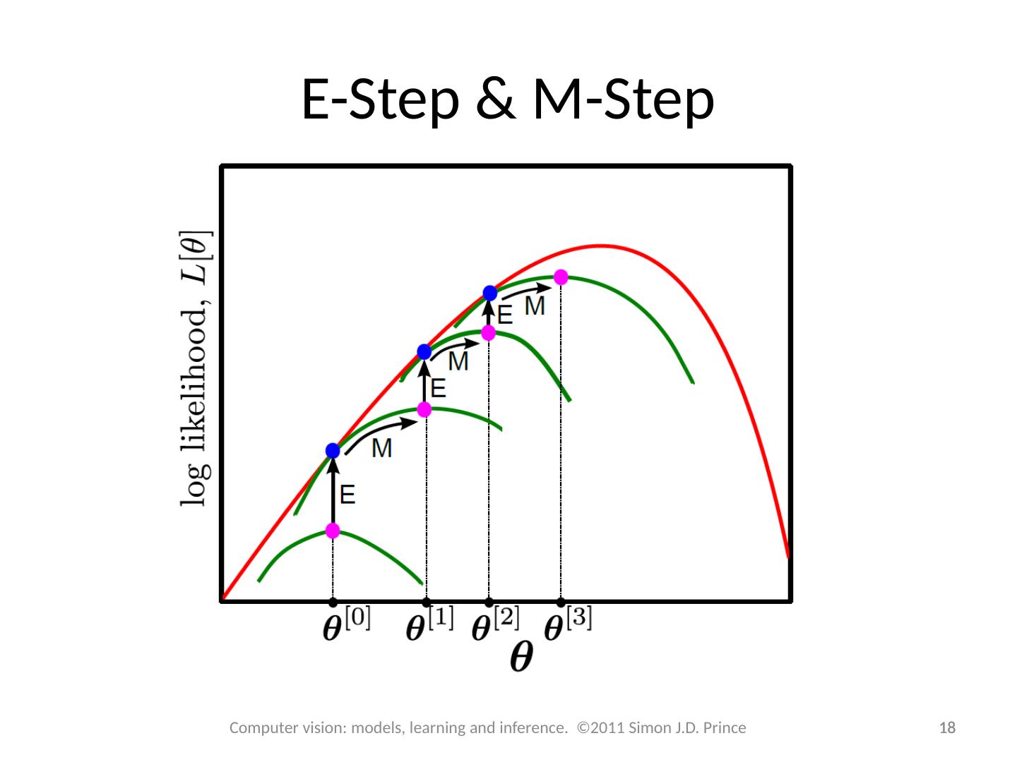
17 .E-Step & M-Step E-Step – Maximize bound w.r.t . distributions q i ( h i ) M-Step – Maximize bound w.r.t . parameters q 17 Computer vision: models, learning and inference. ©2011 Simon J.D. Prince

18 .18 E-Step & M-Step 18 Computer vision: models, learning and inference. ©2011 Simon J.D. Prince

19 .Structure 19 19 Computer vision: models, learning and inference. ©2011 Simon J.D. Prince Densities for classification Models with hidden variables Mixture of Gaussians t-distributions Factor analysis EM algorithm in detail Applications

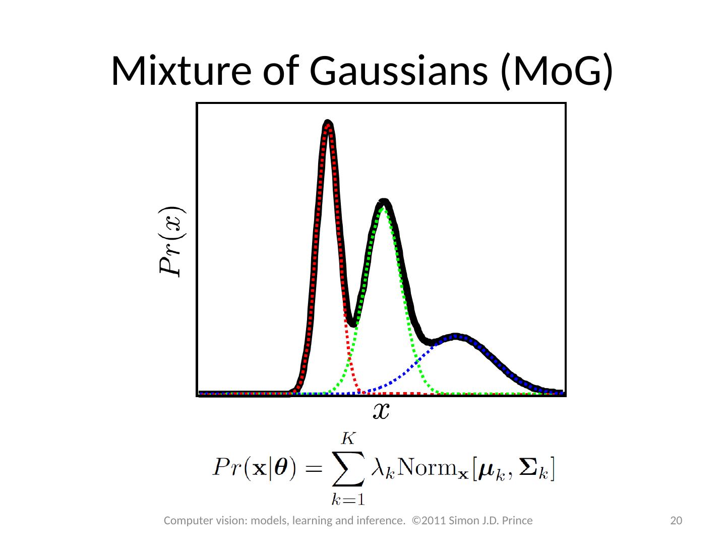
20 .Mixture of Gaussians ( MoG ) 20 Computer vision: models, learning and inference. ©2011 Simon J.D. Prince

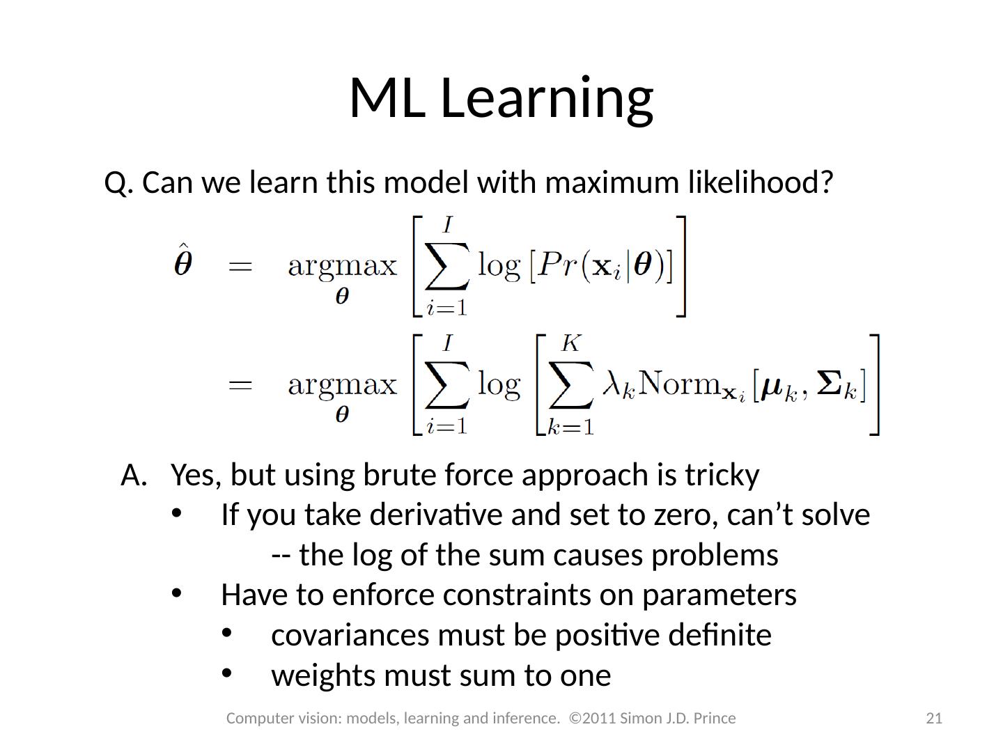
21 .ML Learning Q. Can we learn this model with maximum likelihood? Yes, but using brute force approach is tricky If you take derivative and set to zero, can’t solve -- the log of the sum causes problems Have to enforce constraints on parameters covariances must be positive definite weights must sum to one 21 Computer vision: models, learning and inference. ©2011 Simon J.D. Prince

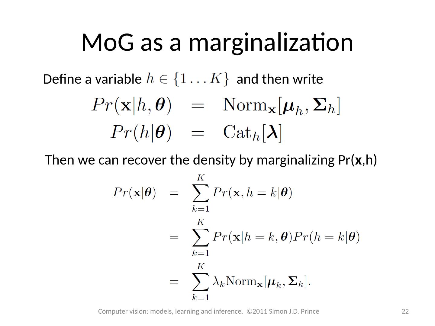
22 .MoG as a marginalization Define a variable and then write Then we can recover the density by marginalizing Pr( x ,h ) 22 Computer vision: models, learning and inference. ©2011 Simon J.D. Prince

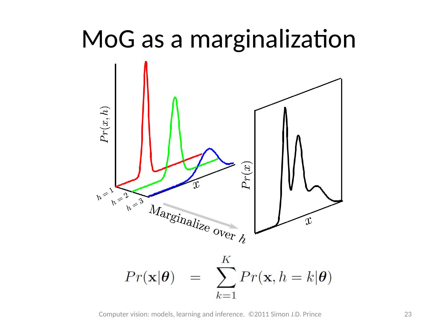
23 .MoG as a marginalization 23 Computer vision: models, learning and inference. ©2011 Simon J.D. Prince

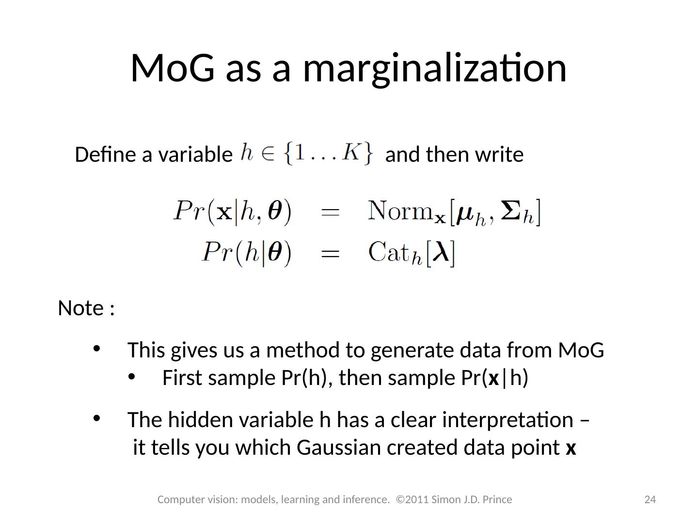
24 .MoG as a marginalization Define a variable and then write Note : This gives us a method to generate data from MoG First sample Pr(h), then sample Pr( x |h ) The hidden variable h has a clear interpretation – it tells you which Gaussian created data point x 24 Computer vision: models, learning and inference. ©2011 Simon J.D. Prince

25 .GOAL: to learn parameters from training data Expectation Maximization for MoG E-Step – Maximize bound w.r.t . distributions q( h i ) M-Step – Maximize bound w.r.t . parameters q 25 Computer vision: models, learning and inference. ©2011 Simon J.D. Prince

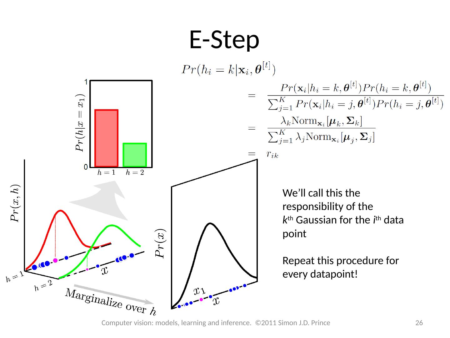
26 .E-Step We’ll call this the responsibility of the k th Gaussian for the i th data point Repeat this procedure for every datapoint ! 26 Computer vision: models, learning and inference. ©2011 Simon J.D. Prince

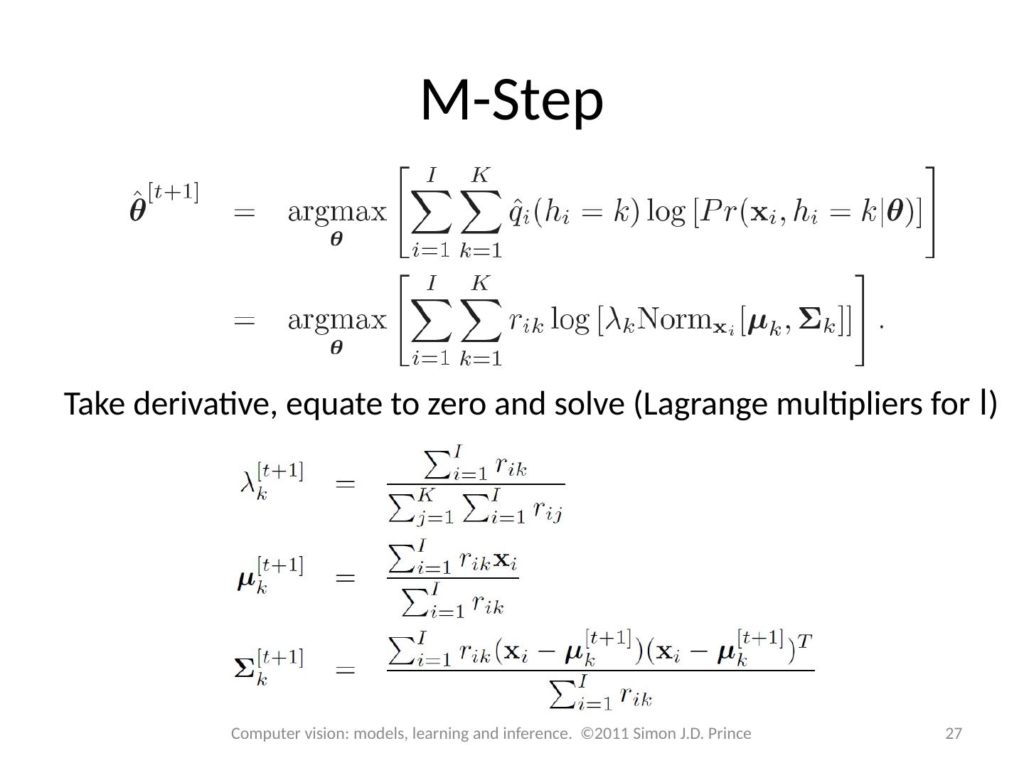
27 .M-Step Take derivative, equate to zero and solve (Lagrange multipliers for l ) 27 Computer vision: models, learning and inference. ©2011 Simon J.D. Prince

28 .M-Step Update means , covariances and weights according to responsibilities of datapoints 28 Computer vision: models, learning and inference. ©2011 Simon J.D. Prince

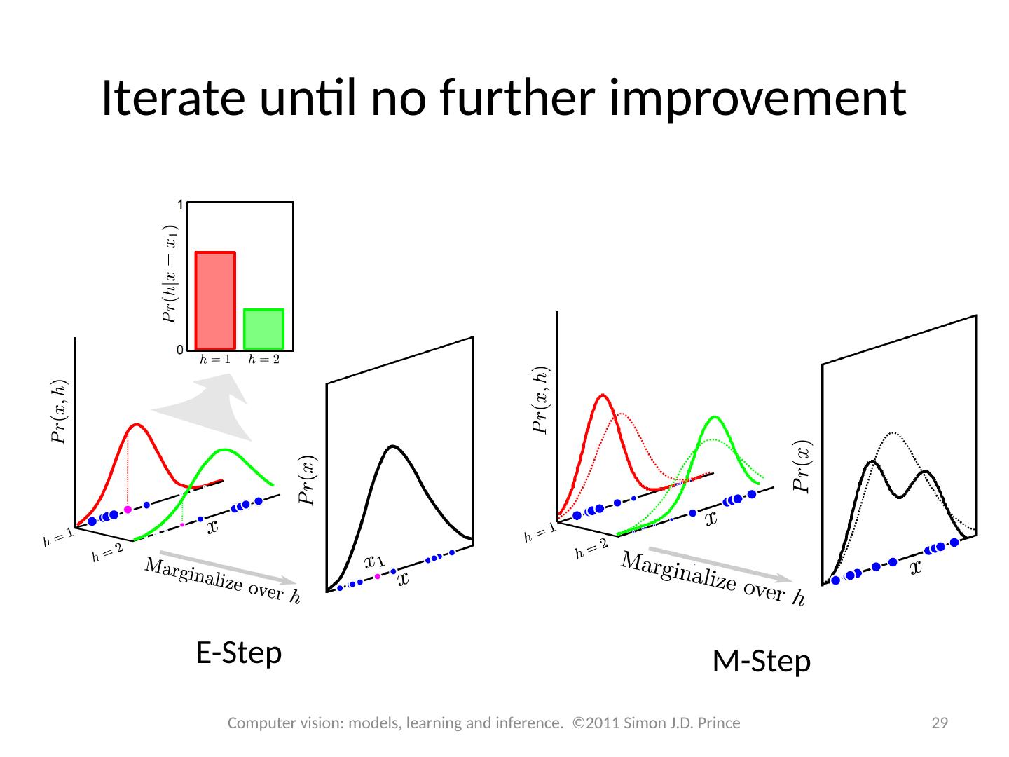
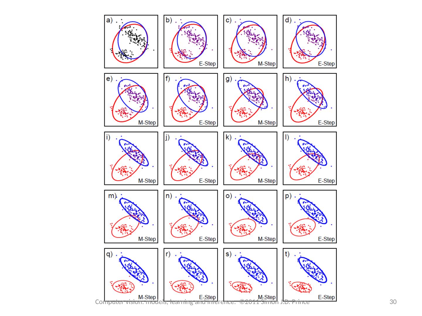
29 .Iterate until no further improvement E-Step M-Step 29 Computer vision: models, learning and inference. ©2011 Simon J.D. Prince