12_Models_For_Grids

1 .Computer vision: models, learning and inference Chapter 12 Models for Grids

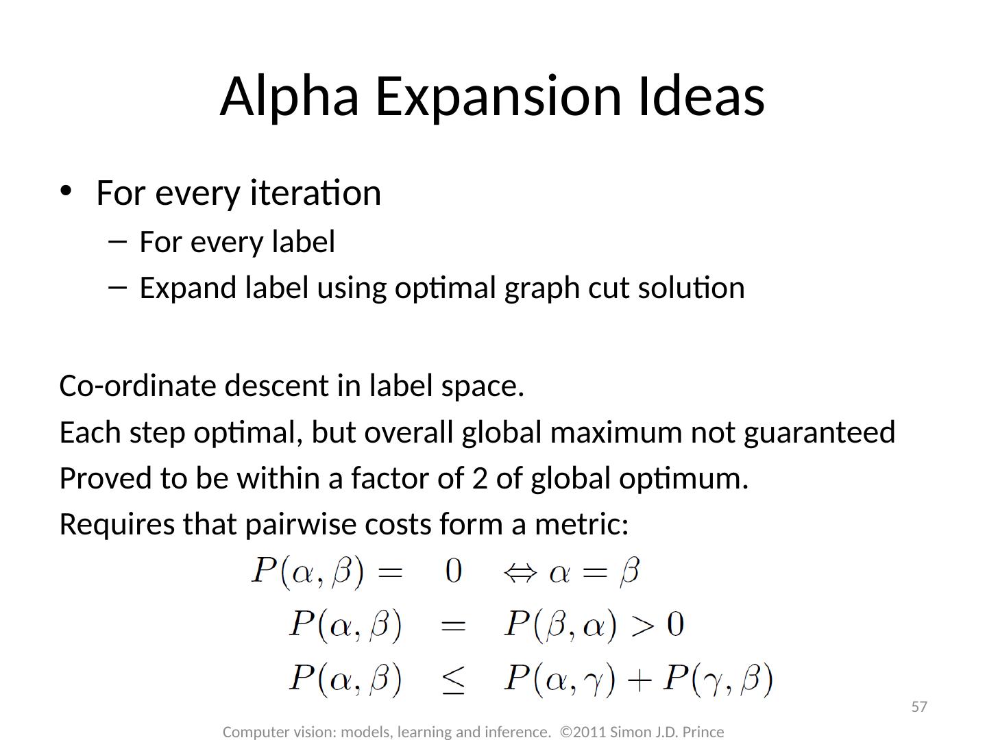
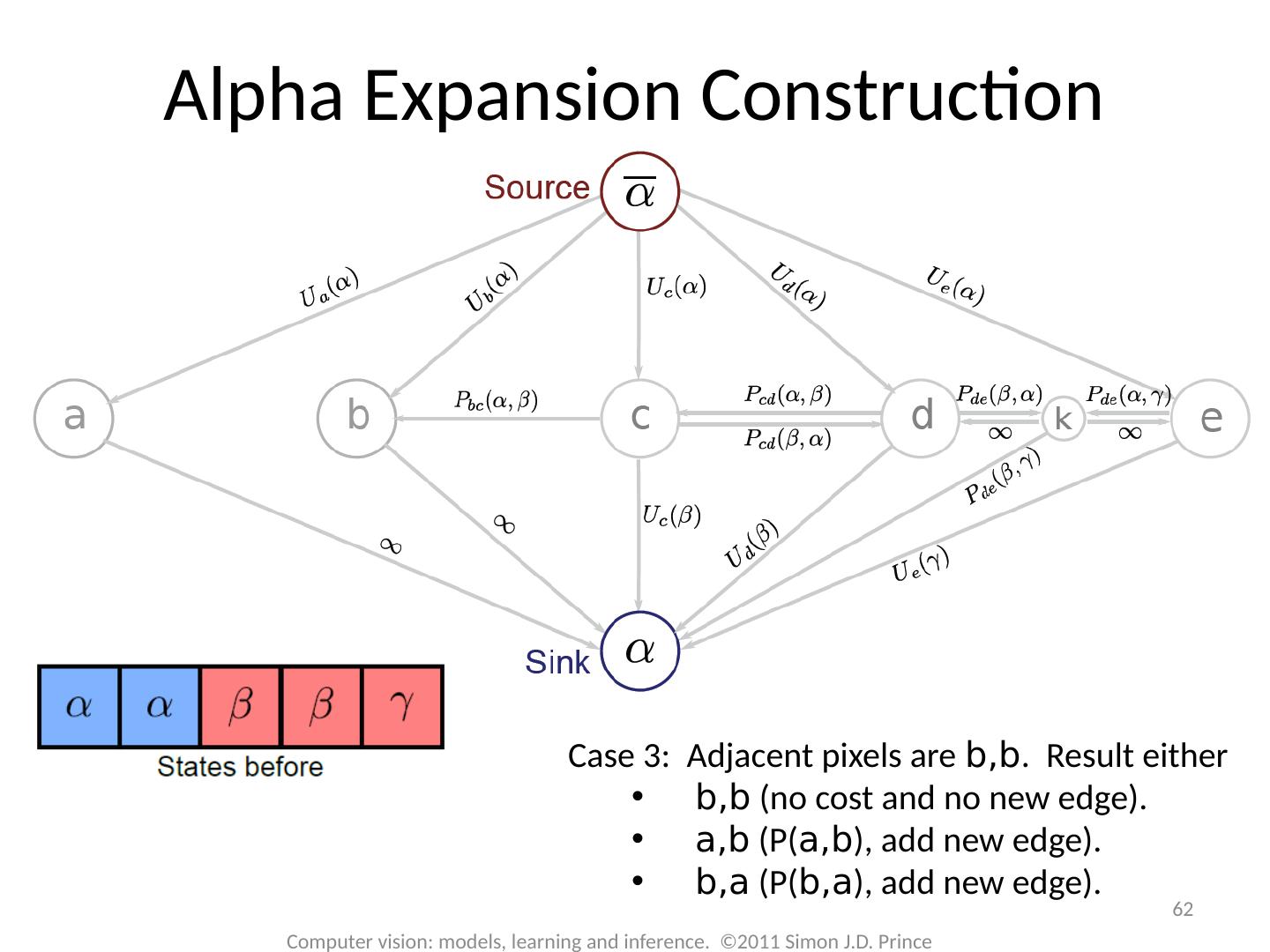
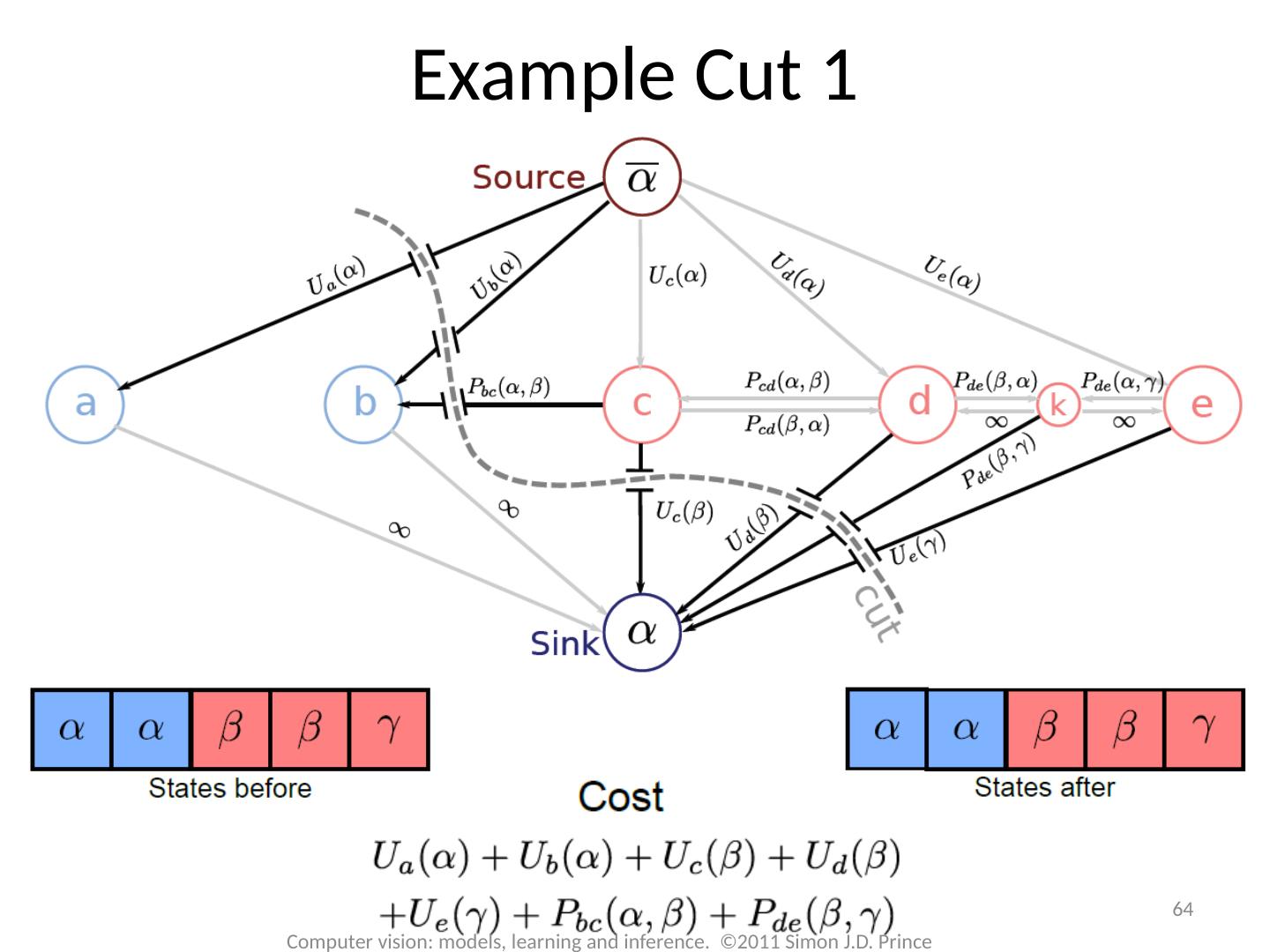
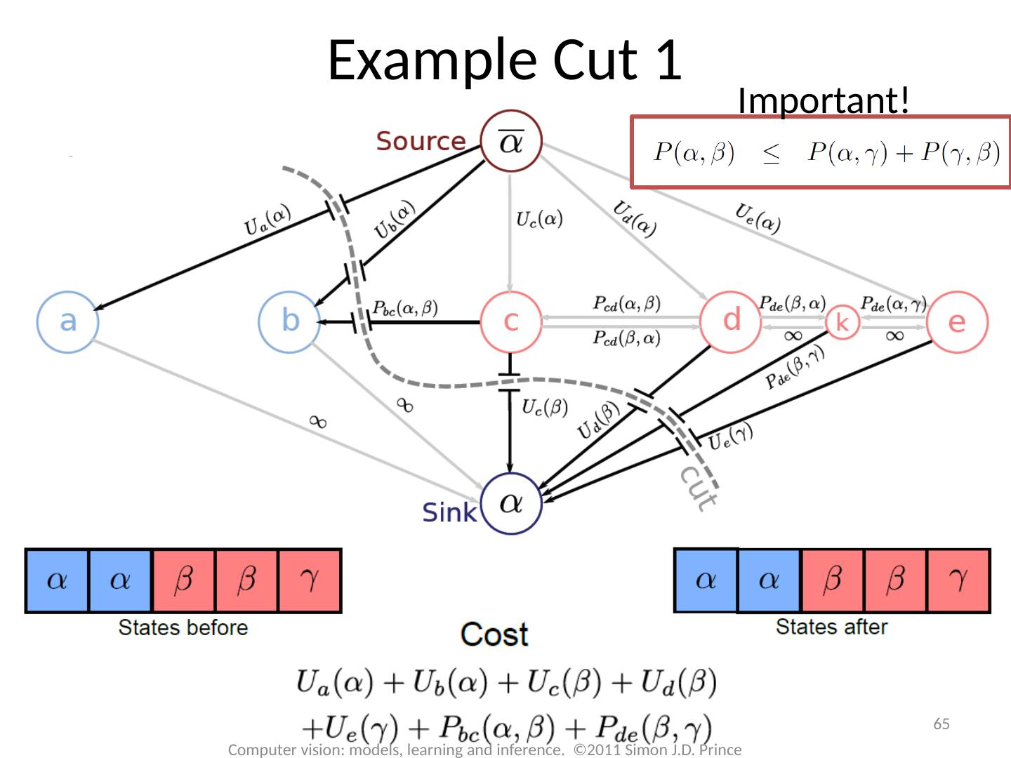
2 .Models for grids 2 Computer vision: models, learning and inference. ©2011 Simon J.D. Prince Consider models with one unknown world state at each pixel in the image – takes the form of a grid . Loops in the graphical model, so cannot use dynamic programming or belief propagation Define probability distributions that favor certain configurations of world states Called Markov random fields Inference using a set of techniques called graph cuts

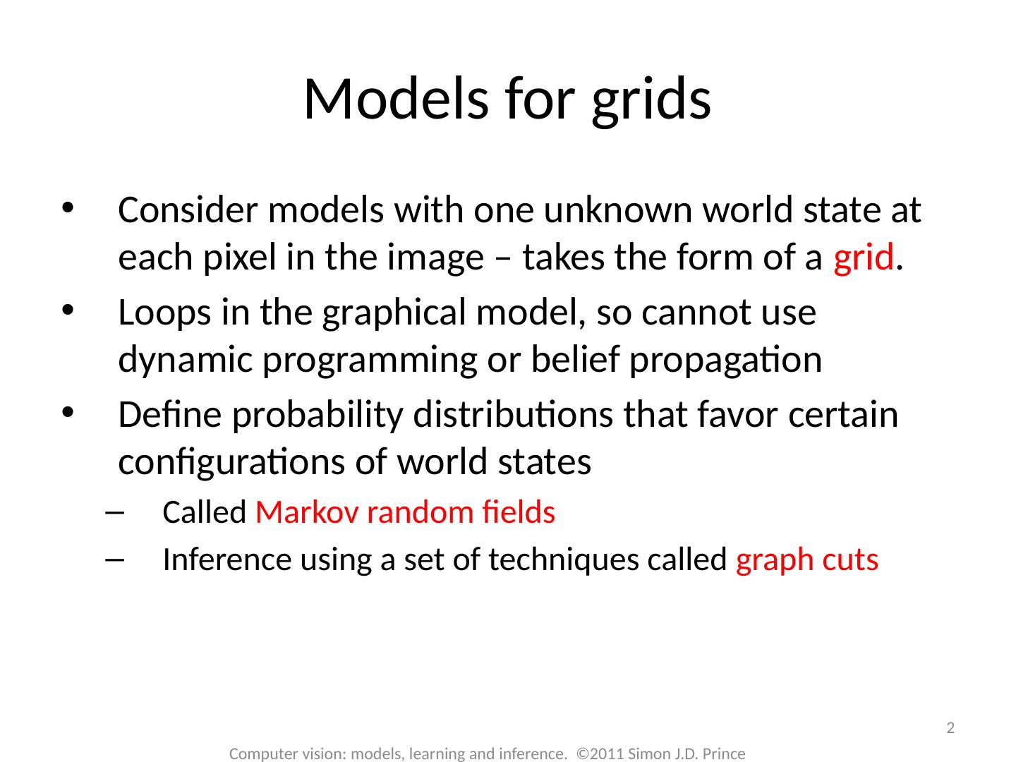
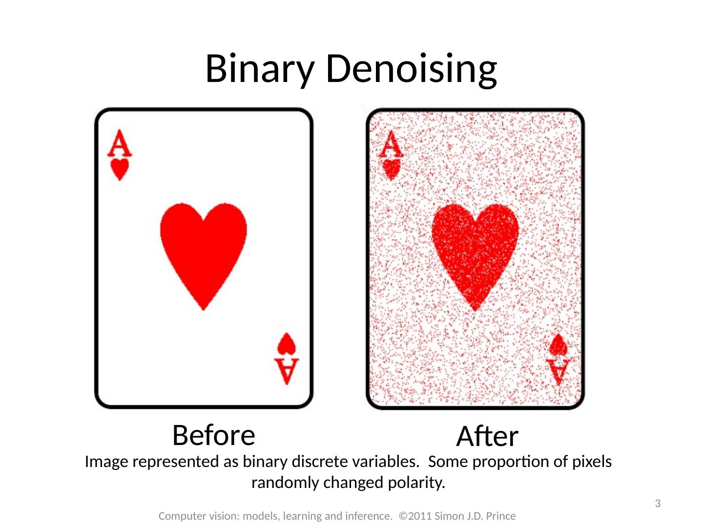
3 .3 Computer vision: models, learning and inference. ©2011 Simon J.D. Prince Binary Denoising Before After Image represented as binary discrete variables. Some proportion of pixels randomly changed polarity.

4 .4 Computer vision: models, learning and inference. ©2011 Simon J.D. Prince Multi-label Denoising Before After Image represented as discrete variables representing intensity. Some proportion of pixels randomly changed according to a uniform distribution.

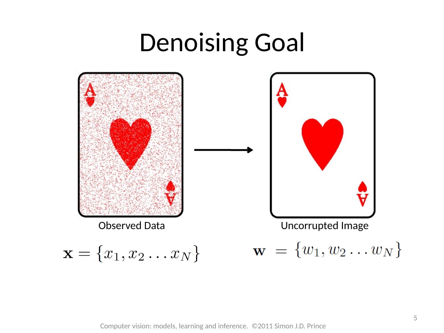
5 .5 Computer vision: models, learning and inference. ©2011 Simon J.D. Prince Denoising Goal Observed Data Uncorrupted Image

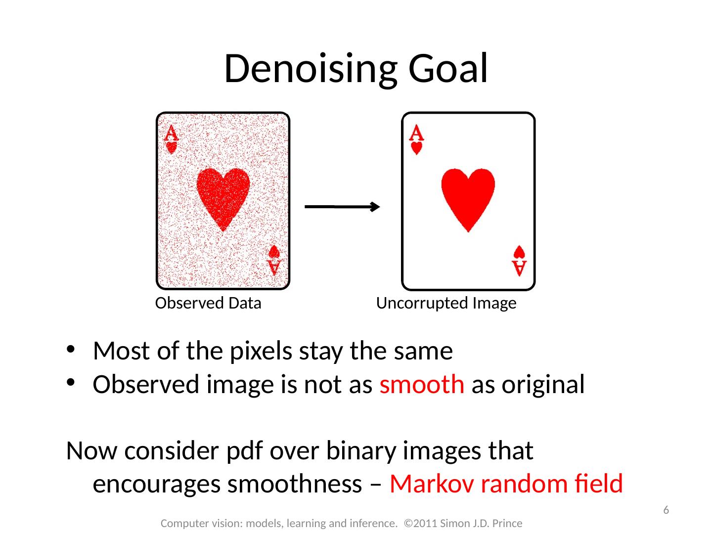
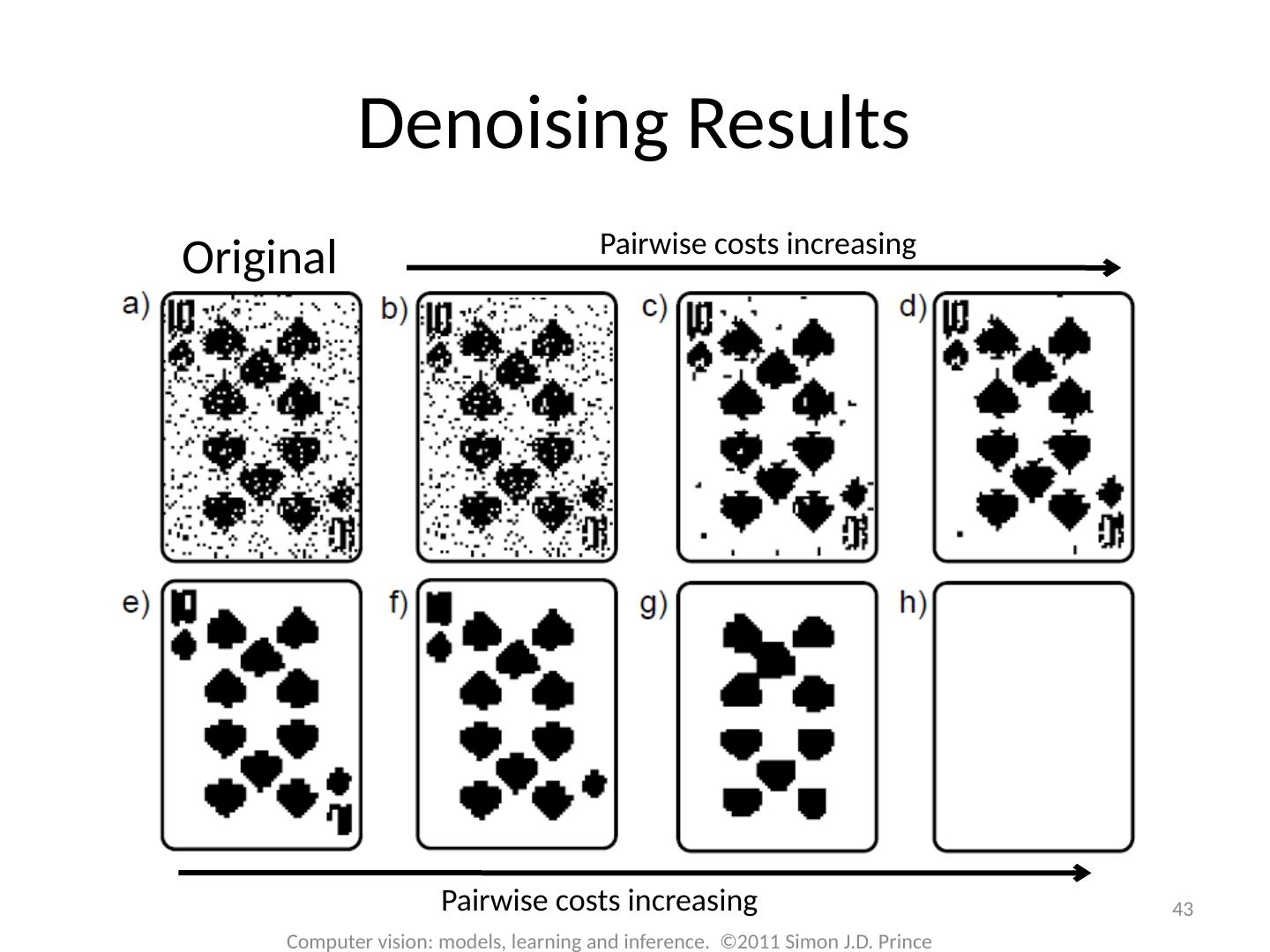
6 .Most of the pixels stay the same Observed image is not as smooth as original Now consider pdf over binary images that encourages smoothness – Markov random field 6 Computer vision: models, learning and inference. ©2011 Simon J.D. Prince Denoising Goal Observed Data Uncorrupted Image

7 .7 Computer vision: models, learning and inference. ©2011 Simon J.D. Prince Markov random fields This is just the typical property of an undirected model. We’ll continue the discussion in terms of undirected models

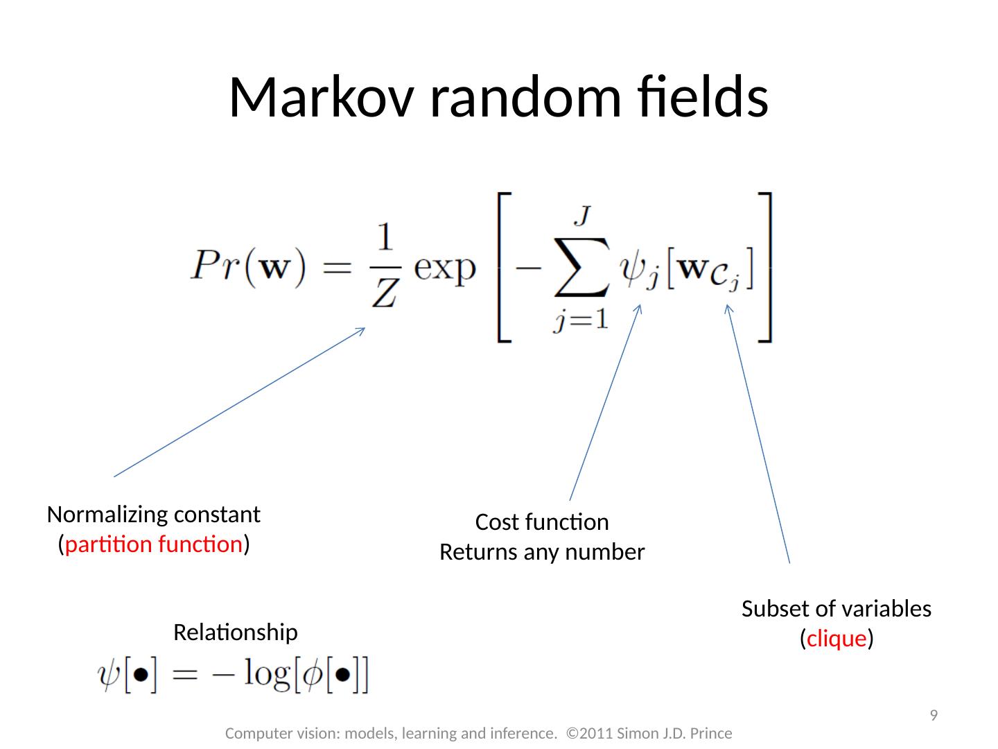
8 .8 Computer vision: models, learning and inference. ©2011 Simon J.D. Prince Markov random fields Normalizing constant ( partition function ) Potential function Returns positive number Subset of variables ( clique )

9 .9 Computer vision: models, learning and inference. ©2011 Simon J.D. Prince Markov random fields Normalizing constant ( partition function ) Cost function Returns any number Subset of variables ( clique ) Relationship

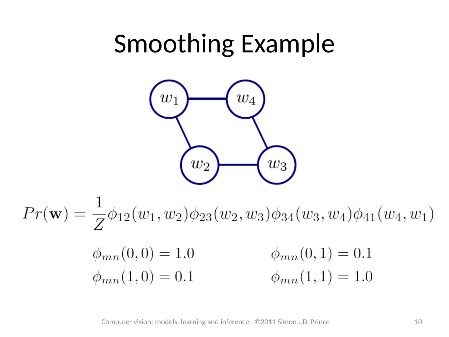
10 .10 Computer vision: models, learning and inference. ©2011 Simon J.D. Prince Smoothing Example

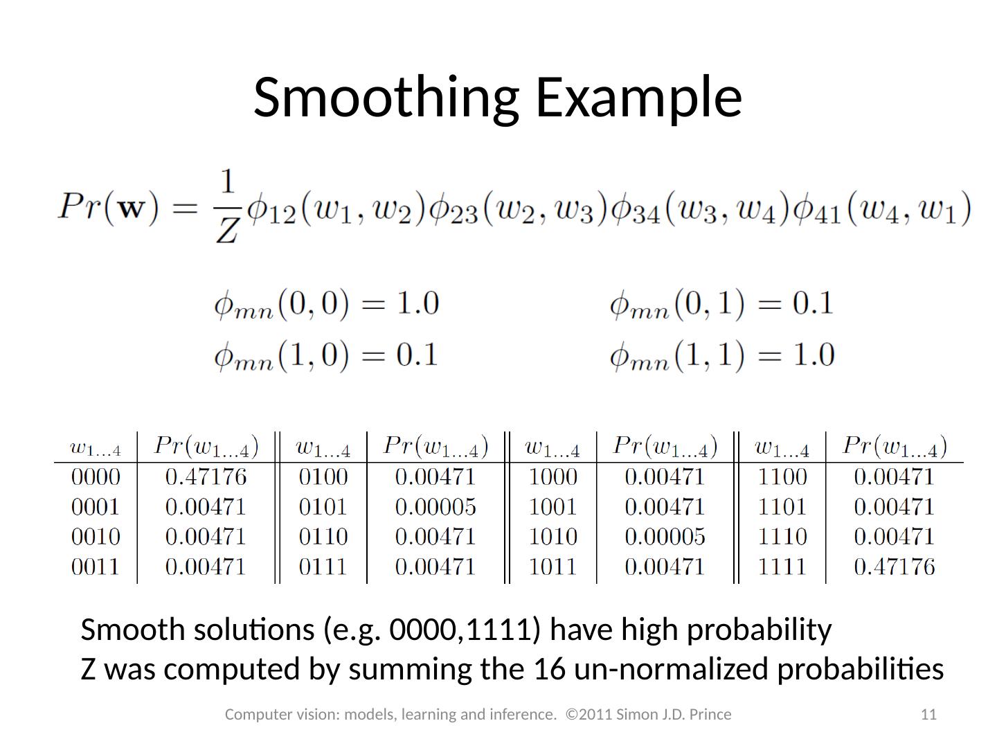
11 .11 Computer vision: models, learning and inference. ©2011 Simon J.D. Prince Smoothing Example Smooth solutions (e.g. 0000,1111) have high probability Z was computed by summing the 16 un-normalized probabilities

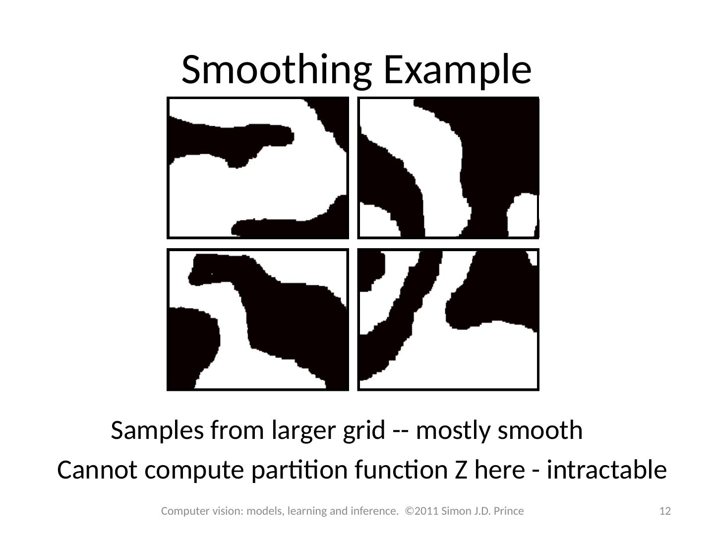
12 .12 Computer vision: models, learning and inference. ©2011 Simon J.D. Prince Smoothing Example Samples from larger grid -- mostly smooth Cannot compute partition function Z here - intractable

13 .13 Computer vision: models, learning and inference. ©2011 Simon J.D. Prince Denoising Goal Observed Data Uncorrupted Image

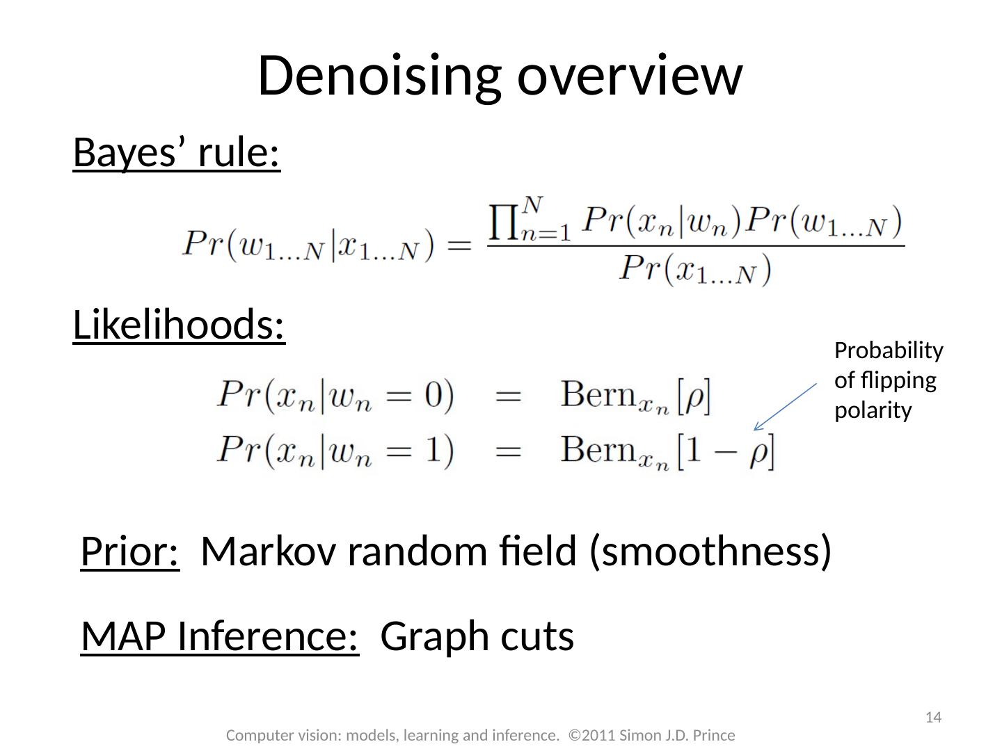
14 .14 Computer vision: models, learning and inference. ©2011 Simon J.D. Prince Denoising overview Bayes ’ rule: Likelihoods: Prior: Markov random field (smoothness) MAP Inference: Graph cuts Probability of flipping polarity

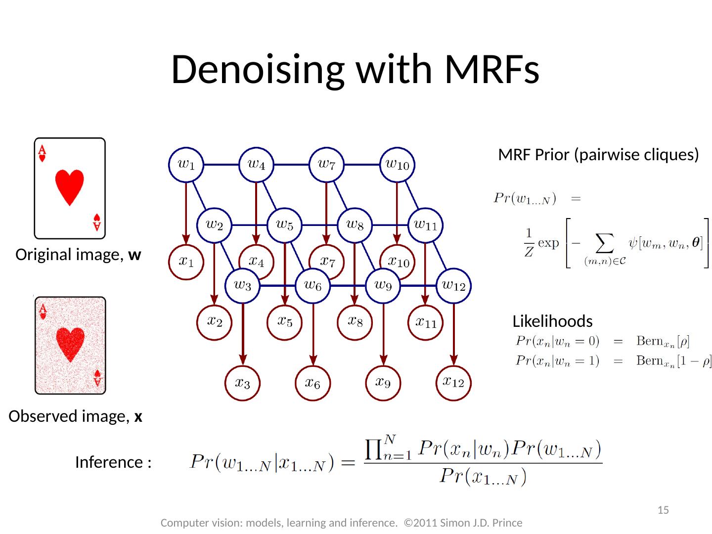
15 .15 Computer vision: models, learning and inference. ©2011 Simon J.D. Prince Denoising with MRFs Observed image, x Original image, w MRF Prior ( pairwise cliques) Inference : Likelihoods

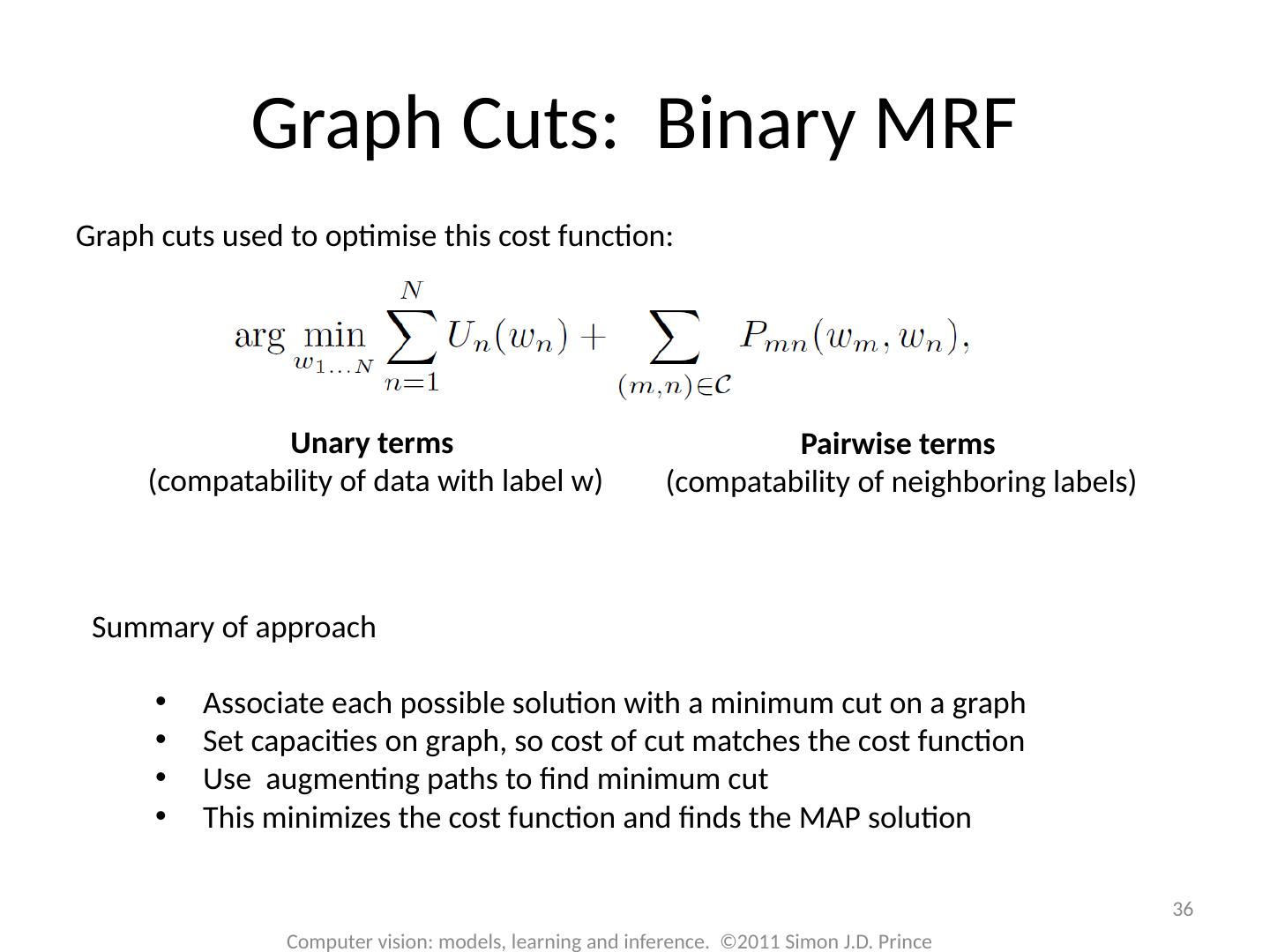
16 .MAP Inference 16 Computer vision: models, learning and inference. ©2011 Simon J.D. Prince Unary terms ( compatability of data with label y) Pairwise terms ( compatability of neighboring labels)

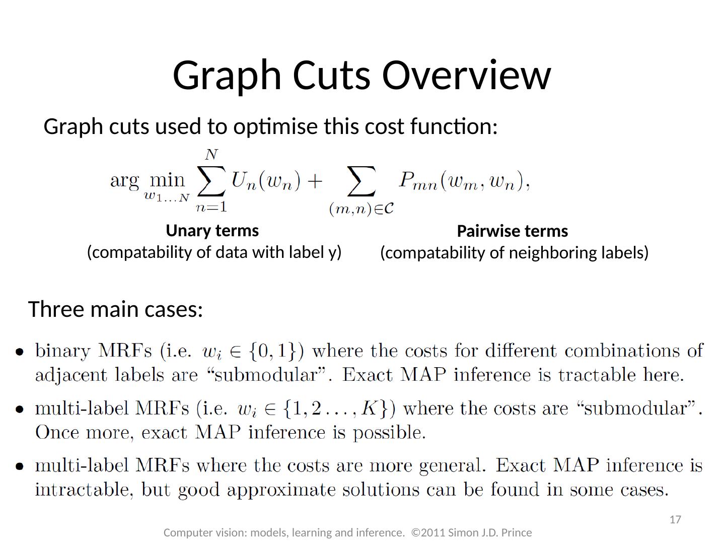
17 .17 Computer vision: models, learning and inference. ©2011 Simon J.D. Prince Graph Cuts Overview Unary terms ( compatability of data with label y) Pairwise terms ( compatability of neighboring labels) Graph cuts used to optimise this cost function: Three main cases:

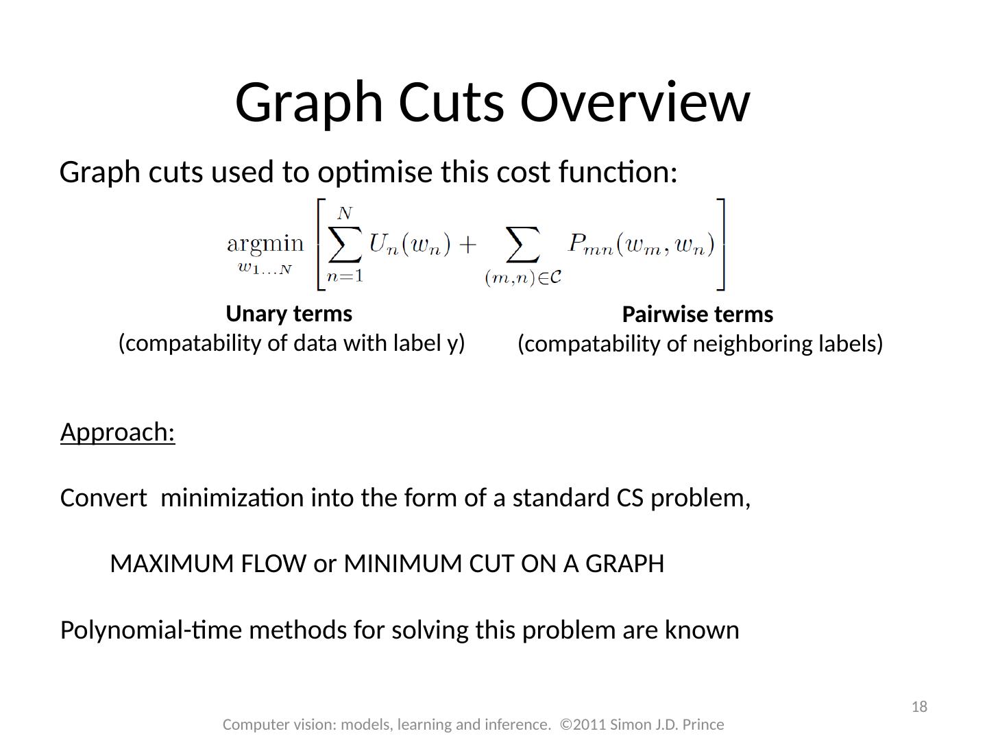
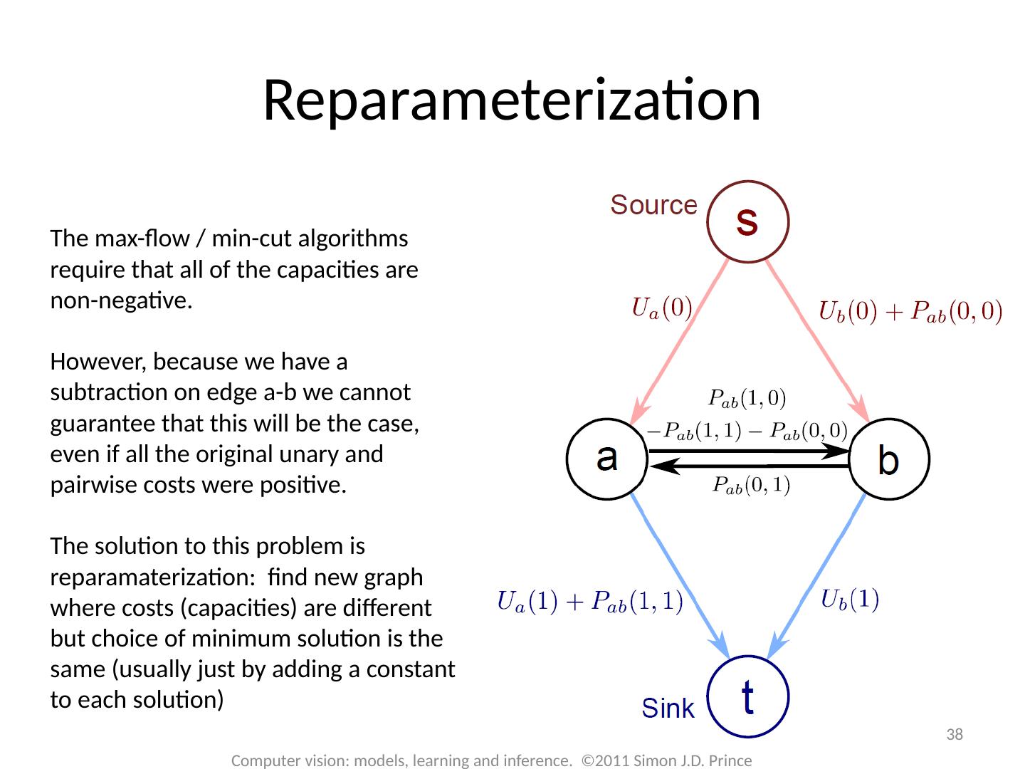
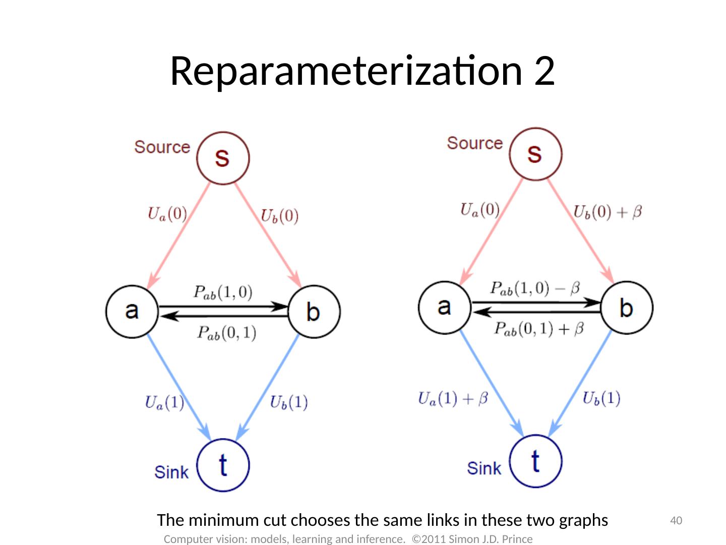
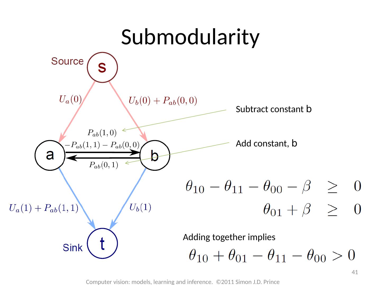
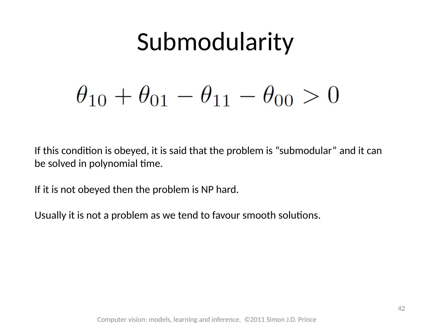
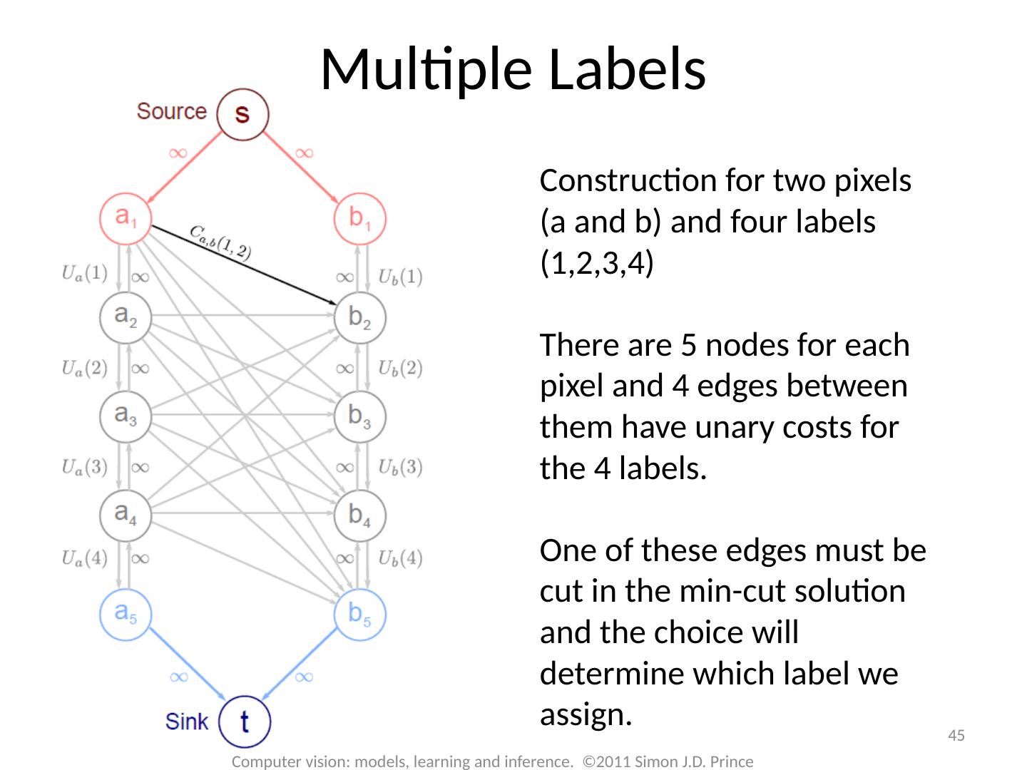
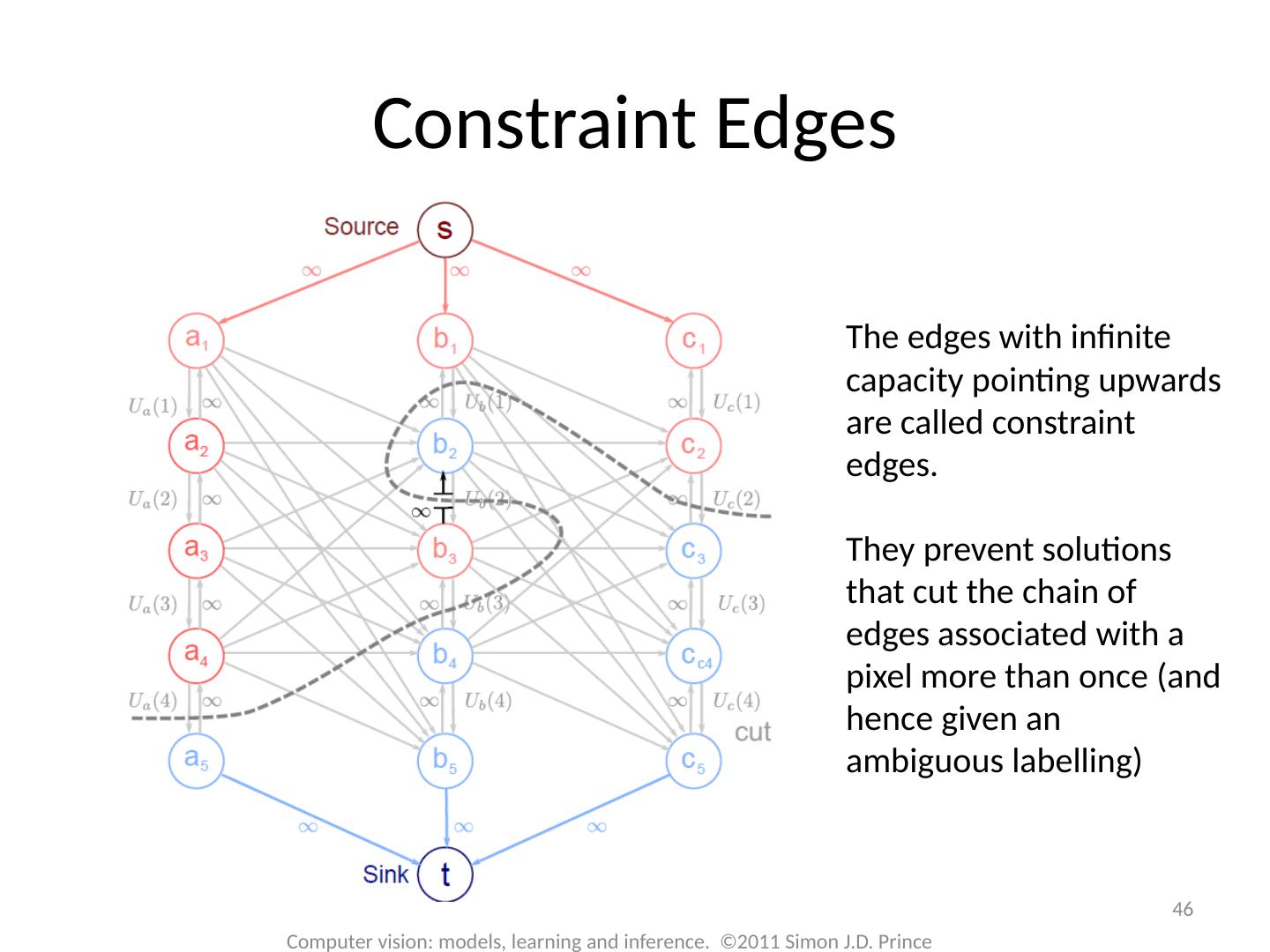
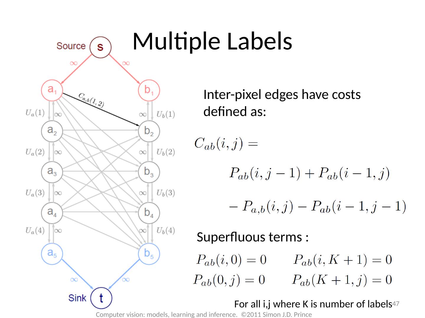
18 .18 Computer vision: models, learning and inference. ©2011 Simon J.D. Prince Graph Cuts Overview Unary terms ( compatability of data with label y) Pairwise terms ( compatability of neighboring labels) Graph cuts used to optimise this cost function: Approach: Convert minimization into the form of a standard CS problem, MAXIMUM FLOW or MINIMUM CUT ON A GRAPH Polynomial-time methods for solving this problem are known

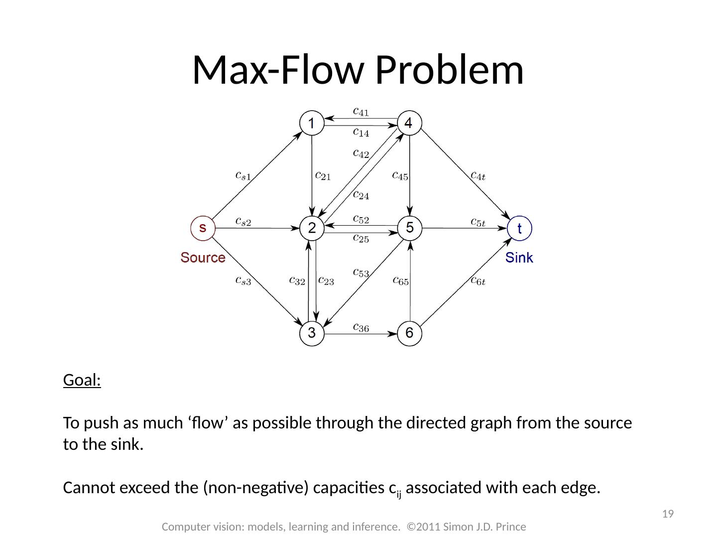
19 .19 Computer vision: models, learning and inference. ©2011 Simon J.D. Prince Max-Flow Problem Goal: To push as much ‘flow’ as possible through the directed graph from the source to the sink. Cannot exceed the (non-negative) capacities c ij associated with each edge.

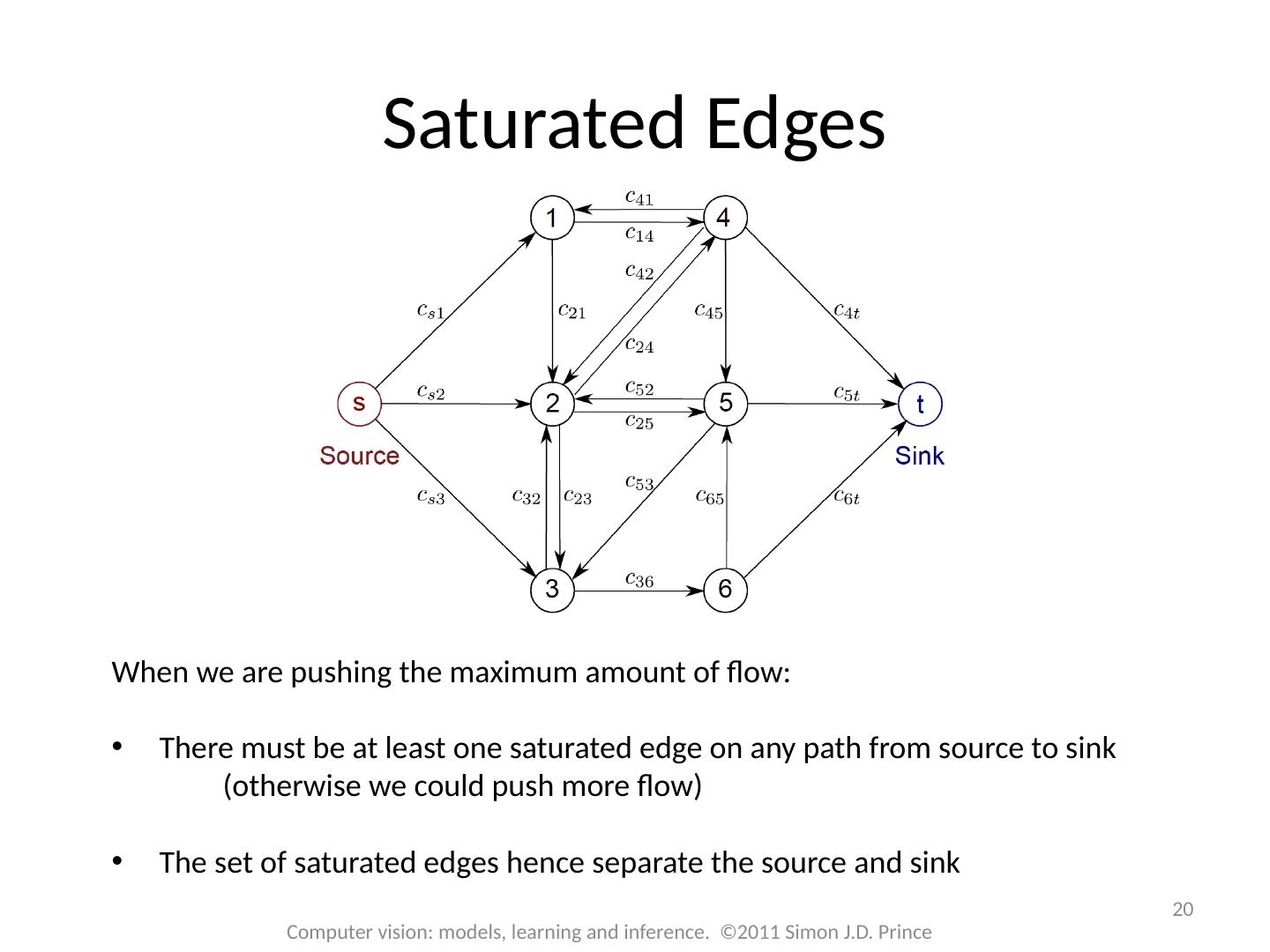
20 .20 Computer vision: models, learning and inference. ©2011 Simon J.D. Prince Saturated Edges When we are pushing the maximum amount of flow: There must be at least one saturated edge on any path from source to sink (otherwise we could push more flow) The set of saturated edges hence separate the source and sink

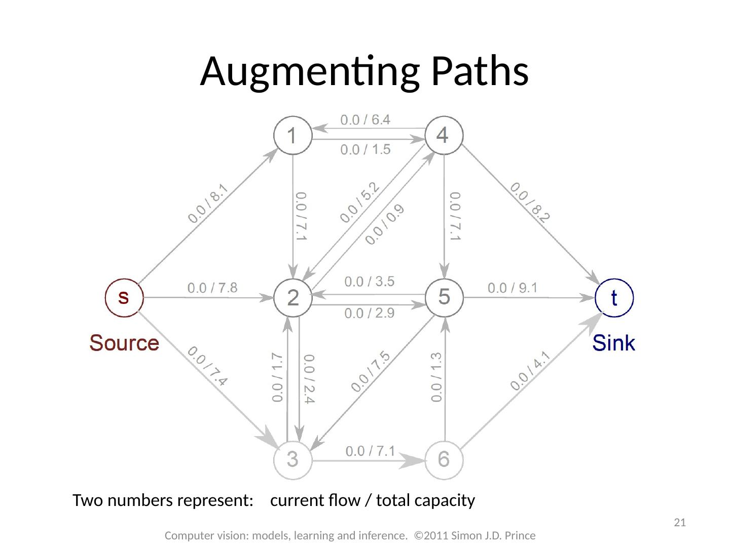
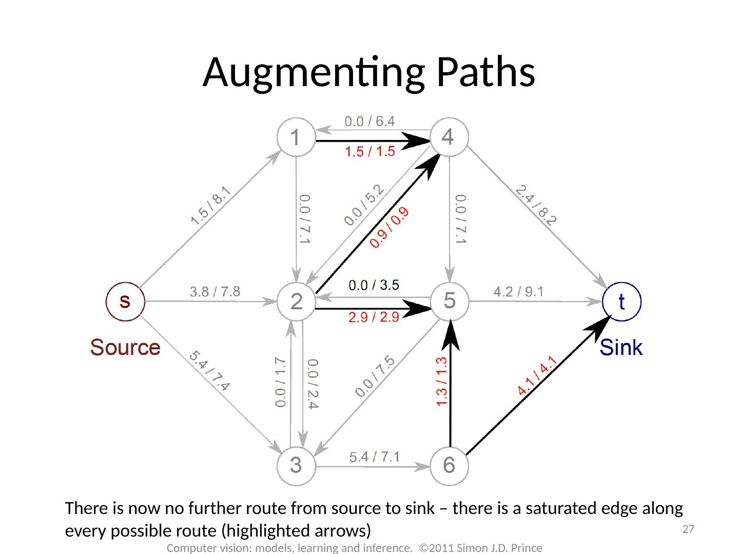
21 .21 Computer vision: models, learning and inference. ©2011 Simon J.D. Prince Augmenting Paths Two numbers represent: current flow / total capacity

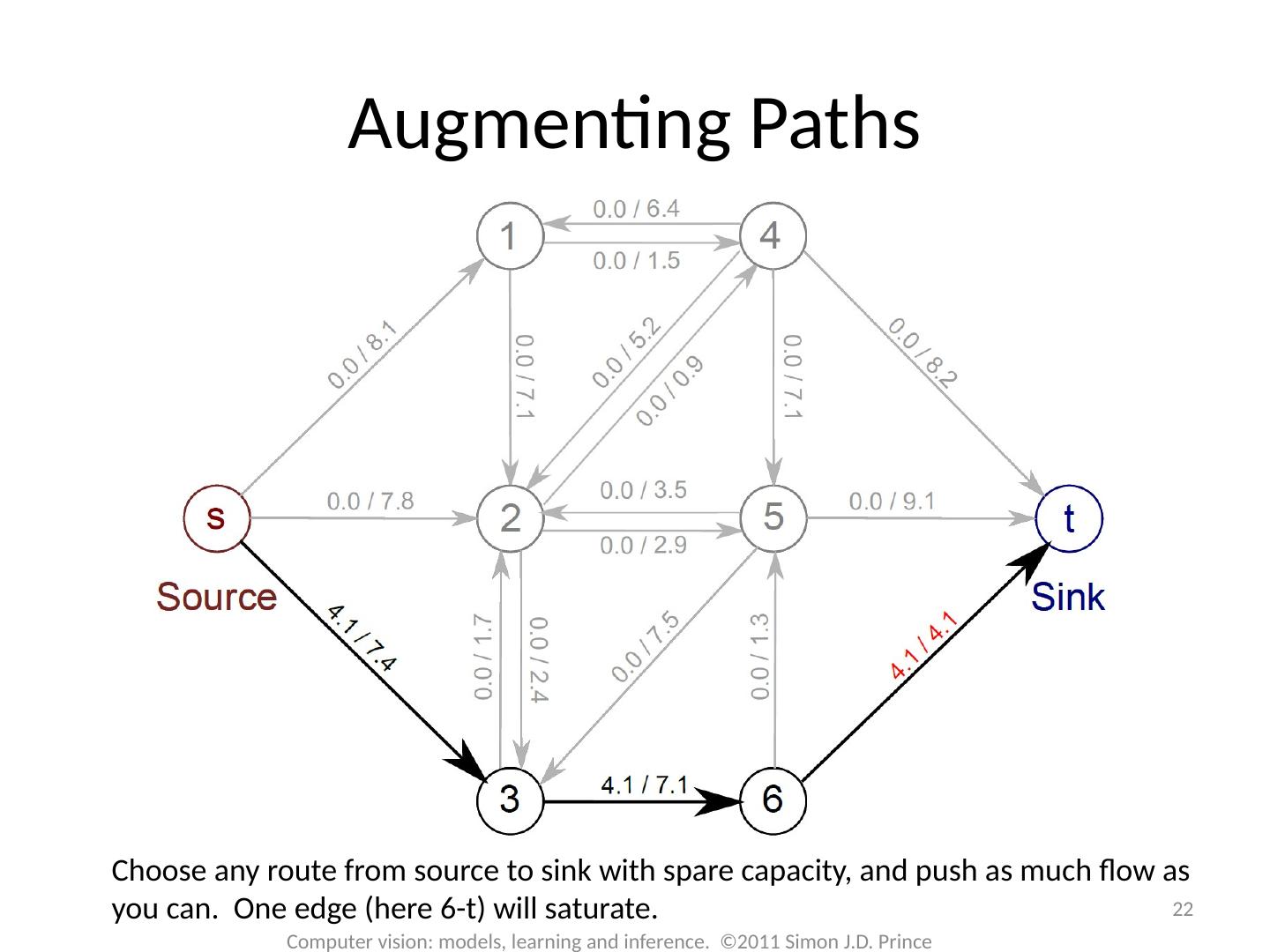
22 .Choose any route from source to sink with spare capacity, and push as much flow as you can. One edge (here 6-t) will saturate. 22 Computer vision: models, learning and inference. ©2011 Simon J.D. Prince Augmenting Paths

23 .23 Computer vision: models, learning and inference. ©2011 Simon J.D. Prince Augmenting Paths Choose another route, respecting remaining capacity. This time edge 6-5 saturates.

24 .24 Computer vision: models, learning and inference. ©2011 Simon J.D. Prince Augmenting Paths A third route. Edge 1-4 saturates

25 .25 Computer vision: models, learning and inference. ©2011 Simon J.D. Prince Augmenting Paths A fourth route. Edge 2-5 saturates

26 .26 Computer vision: models, learning and inference. ©2011 Simon J.D. Prince Augmenting Paths A fifth route. Edge 2-4 saturates

27 .There is now no further route from source to sink – there is a saturated edge along every possible route (highlighted arrows) 27 Computer vision: models, learning and inference. ©2011 Simon J.D. Prince Augmenting Paths

28 .28 Computer vision: models, learning and inference. ©2011 Simon J.D. Prince Augmenting Paths The saturated edges separate the source from the sink and form the min-cut solution. Nodes either connect to the source or connect to the sink.

29 .Graph Cuts: Binary MRF Unary terms ( compatability of data with label w) Pairwise terms ( compatability of neighboring labels) Graph cuts used to optimise this cost function: First work with binary case (i.e. True label w is 0 or 1) Constrain pairwise costs so that they are “zero-diagonal” Computer vision: models, learning and inference. ©2011 Simon J.D. Prince 29