Training Deep Neural Networks

1 .

2 .Getting complex This slide deck begins to consider ML models containing: 10+ layers Each layer with hundreds of neurons A model with hundreds of thousands of connections

3 .challenges Vanishing Gradients Exploding Gradients Both affect DNN and make lower layers difficult to train Training may take a lot of time Millions of parameters risk overfitting the training data set

4 .Backpropagation Backpropagation works its way from the output later (reverse) to the input later- propagating the error gradient on the way. Having computed the gradient of the cost function for each parameter in the network- it utilizes these gradients to update each parameter with a Gradient Descent step.

5 .Vanishing Gradients Issue: Gradients often get continually smaller as the learning algorithms progress down to lower layers. Problem: The Gradient Descent updates leaves the lower layer connection weights virtually unchanged. Result: The training never converges to a good solution. This is called the VANISHING GRADIENT problem.

6 .Exploding Gradients Issue: Sometimes gradients can grow bigger as the learning algorithms progress- this is mostly encountered in Recurrent Neural Networks. (RNN) Problem: Many layers get insanely large weight updates Result: The training algorithm diverges for an optimal solution. This is called the EXPLODING GRADIENT problem.

7 .Abandoned and then re-considered The vanishing  and exploding  gradient issues resulted in neural network research being abandoned for a long time. 2010 - "Understanding the Difficulty of Training Deep Feedforward Neural Networks" was published by Xavier Glorot and Yoshua Begio .

8 .THe suspects Popular use of the sigmoid activation function. Weight initialization scheme using random values using a mean of 0 and standard deviation of 1.

9 .Decoding the problem Utilizing the sigmoid activation function and initialization scheme resulted in the variance of the outputs of each layer is much greater than the inputs. The variance continues increasing after each layer until the activation function saturates at the top layers. This is further aggravated by the fact that the logistic function has a mean of 0.5 not 0.

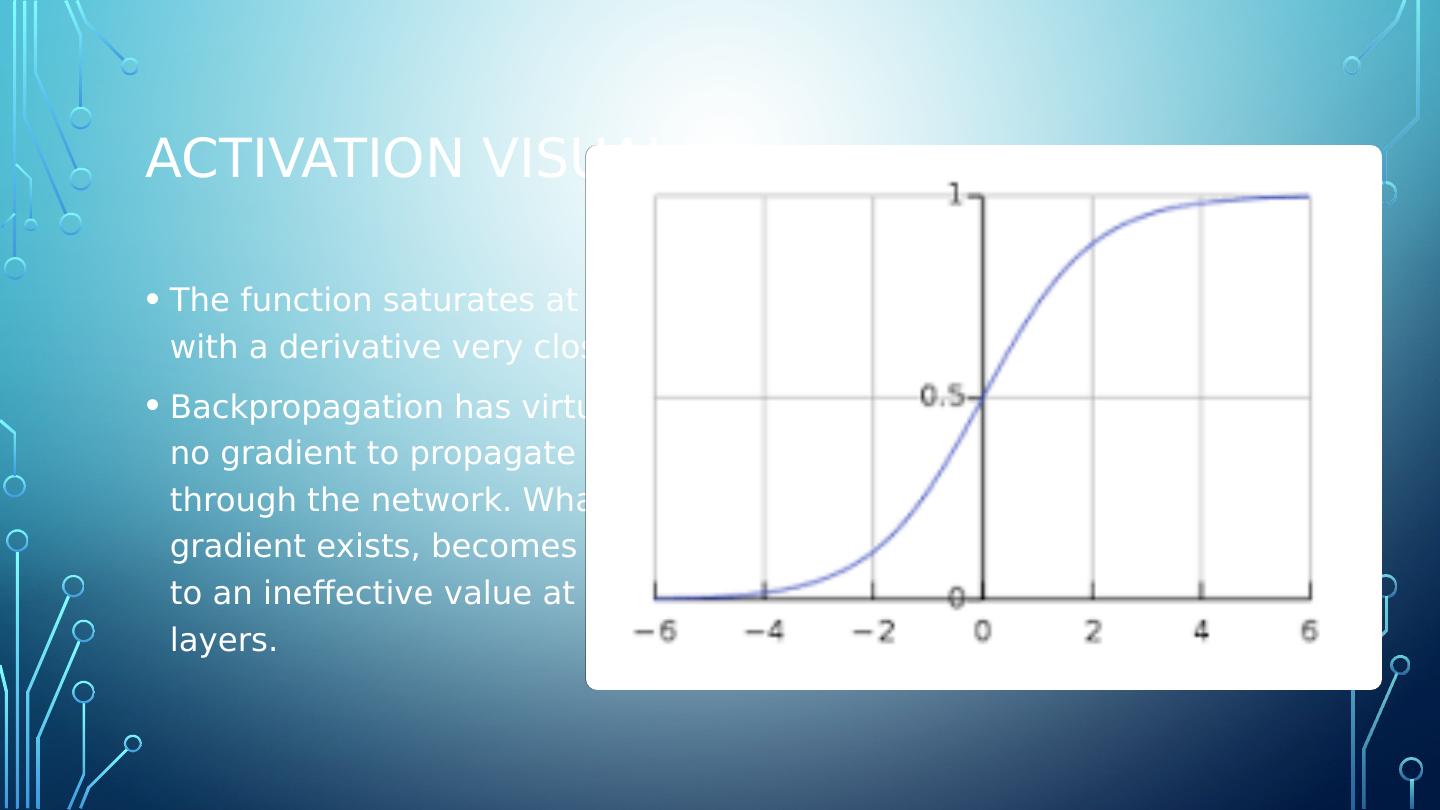
10 .Activation visual The function saturates at 0 or 1 with a derivative very close to 0. Backpropagation has virtually no gradient to propagate back through the network. What little gradient exists, becomes diluted to an ineffective value at lower layers.

11 .Xavier and He proposal The signal needs to flow properly in both directions- forward when predicting and in reverse during backpropagation of gradients. The signal should not die out. The signal should not explode or saturate. The variance of the outputs of each layer need to be equal to the variance of the inputs. The gradients need to have equal variance before and after flowing through a layer in the reverse direction.

12 .Proposal compromise Guaranteeing equal variance through a layer and equal variance of outputs from inputs. This is typically NOT possible unless the layer has an equal number of inputs and outputs. Solution: The connection weights must be initialized randomly. This initialization strategy is often referred to as Xavier Initialization.

13 .Proposal compromise Guaranteeing equal variance through a layer and equal variance of outputs from inputs. This is typically NOT possible unless the layer has an equal number of inputs and outputs. Solution: The connection weights must be initialized randomly. This initialization strategy is often referred to as Xavier Initialization.

14 .Proposal compromise Guaranteeing equal variance through a layer and equal variance of outputs from inputs. This is typically NOT possible unless the layer has an equal number of inputs and outputs. Solution: The connection weights must be initialized randomly. This initialization strategy is often referred to as Xavier Initialization.

15 .Nonsaturating activation functions The Glorot and Bengio  paper of 2010 identified the poor choice in selecting a biologically inspired activation function- sigmoid. However ReLU (Rectified Linear Unit) activation functions tend to be a better choice.

16 .JUMP TO the Activation function slide deck

17 .Batch normalization Though the various random initialization strategies presented earlier can initially reduce the vanishing/exploding gradient training problem... it doesnt guarantee that the issue wont come back during later training. A 2015 paper by Ioffe and Szegedy proposed a technique called Batch Normalization (BN) , addressing the vanishing/exploding gradient issue later in training.

18 .Scaling and shifting Batch Normalization consists of adding an operation in the model before the activation function of each layer. The function zero-centers and normalizes the inputs, then scales and shifts the result utilizing two new parameters per layer. (scaling and shifting values) This operation lets the model learn the optimal scale and mean of the inputs for each layer. The whole training set must be utilized to compute the mean and standard deviation. (There is no mini-batch way of doing this.)

19 .Batch Normalization in use The vanishing gradients problem was strongly reduced (to the point where saturating activation functions can be used). Removes the need for normalization of the input data. The model networks are much less sensitive to weight initialization. Much larger learning rates may be applied, speeding up the learning process.  Batch Normalization acts as a regularizer - which penalizes the loss function and reduces overfitting .

20 .Batch normalization penalty Adds some additional complexity to the model. Neural networks will make slower predictions (due to the extra computations necessary at each layer.)

21 .Batch Normalization in Code See Jupyter Notebook...

22 .Gradient clipping Though this technique has fallen out of favor since Batch Normalization was introduced... a once popular technique to deal with exploding gradients was to simply clip the gradients during backpropagation so they never exceeded a predetermined threshold. TensorFlow provides the clip_by_value  function to perform the clipping function.

23 .Reusing pretrained layers It is always a good idea to try to locate an existing neural network that accomplishes a similar task, and re-using it, before endeavoring to train a very large DNN from scratch. Reuse the lower layers of the pre-trained neural network. This is known as transfer learning. Greatly speeds up the training process. Requires much less training data.

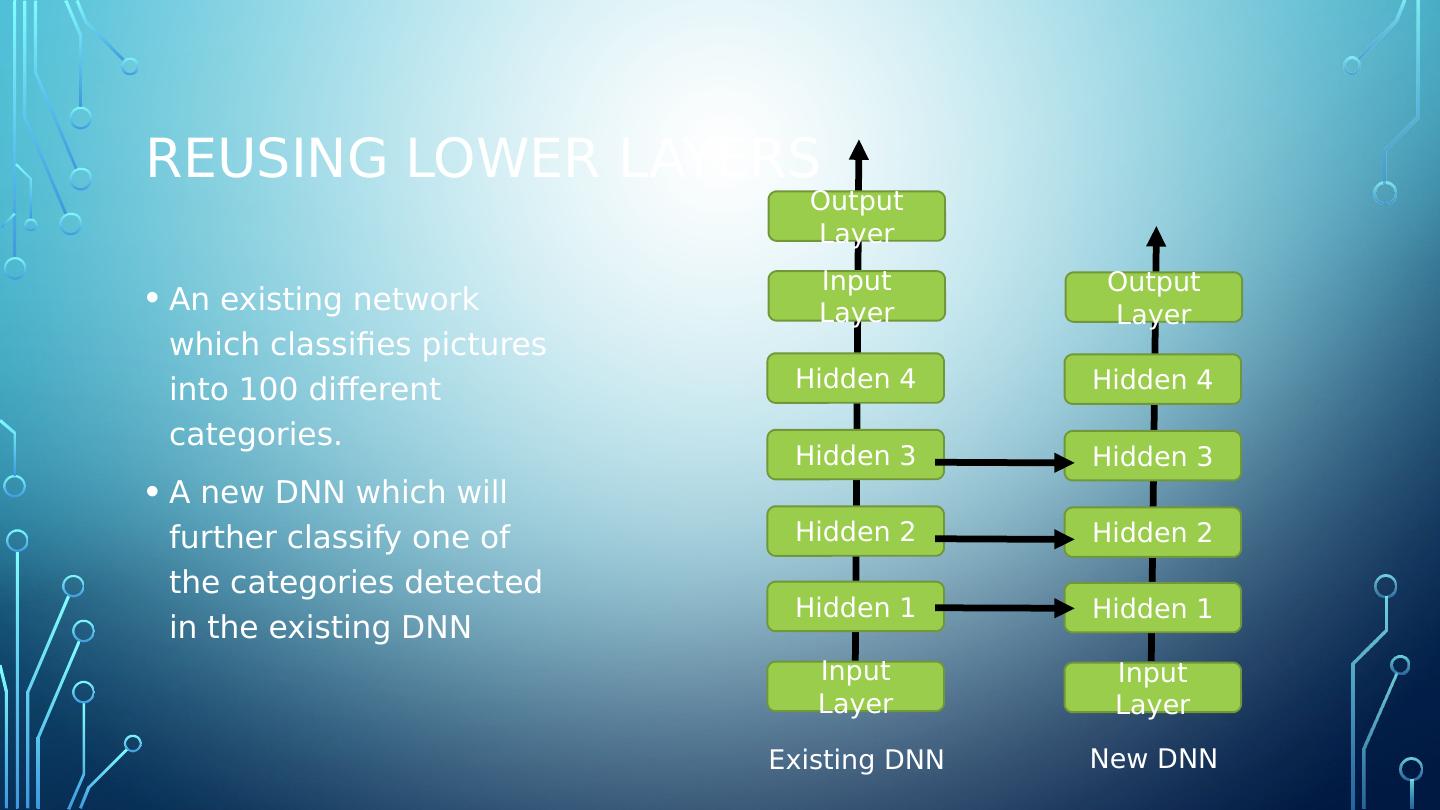
24 .Reusing lower layers An existing network which classifies pictures into 100 different categories. A new DNN which will further classify one of the categories detected in the existing DNN Input Layer Hidden 1 Hidden 2 Hidden 3 Hidden 4 Input Layer Output Layer Input Layer Hidden 1 Hidden 2 Hidden 3 Hidden 4 Output Layer Existing DNN New DNN

25 .Model reuse tip The inputs to the model for which you are borrowing the layers of an existing model must be the same. For example, if the model classifies the contents of a specific size image, your model must provide images the same size.

26 .Model reuse tip The inputs to the model for which you are borrowing the layers of an existing model must be the same. For example, if the model classifies the contents of a specific size image, your model must provide images the same size.

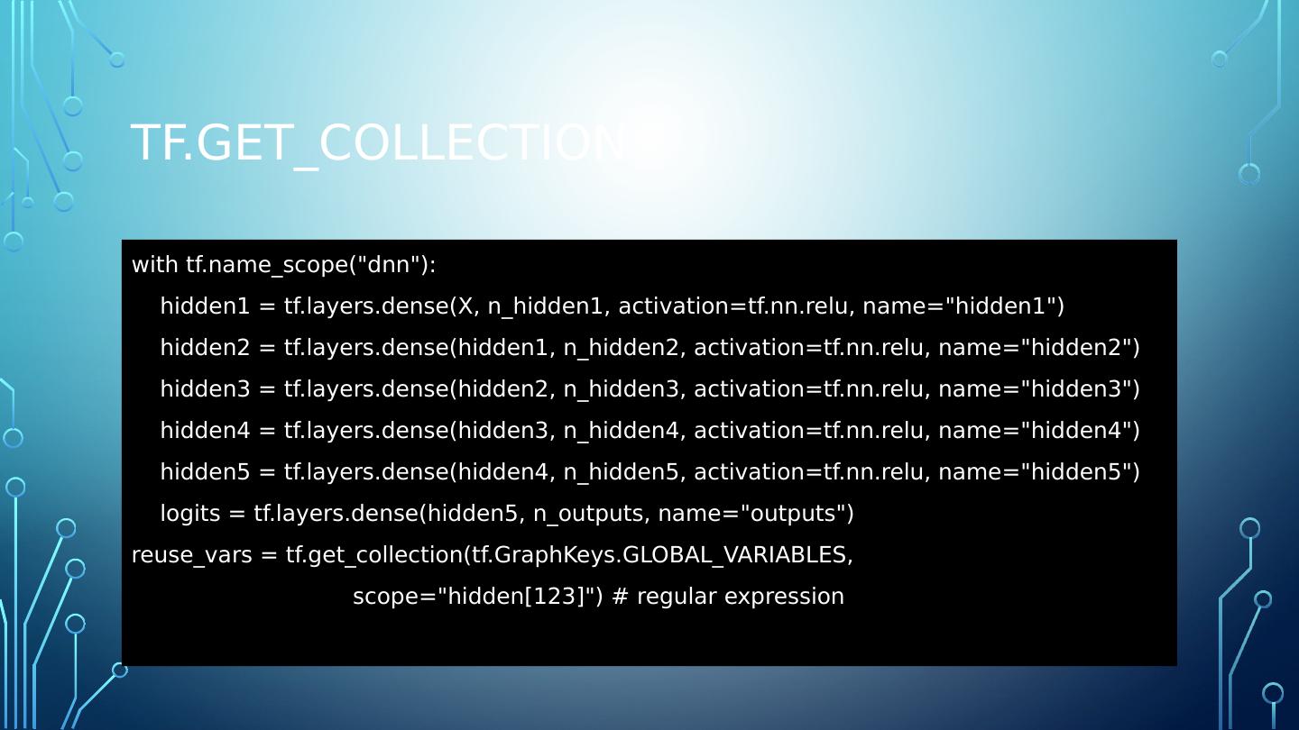
27 .Tf.get_collection with tf.name_scope (" dnn "):     hidden1 = tf.layers.dense(X, n_hidden1, activation=tf.nn.relu, name="hidden1")     hidden2 = tf.layers.dense(hidden1, n_hidden2, activation=tf.nn.relu, name="hidden2")     hidden3 = tf.layers.dense(hidden2, n_hidden3, activation=tf.nn.relu, name="hidden3")     hidden4 = tf.layers.dense(hidden3, n_hidden4, activation=tf.nn.relu, name="hidden4")     hidden5 = tf.layers.dense(hidden4, n_hidden5, activation=tf.nn.relu, name="hidden5")     logits = tf.layers.dense (hidden5, n_outputs , name="outputs") reuse_vars = tf.get_collection ( tf.GraphKeys.GLOBAL_VARIABLES ,                                scope="hidden[123]") # regular expression

28 .Tf.get_collection with tf.name_scope (" dnn "):     hidden1 = tf.layers.dense(X, n_hidden1, activation=tf.nn.relu, name="hidden1")     hidden2 = tf.layers.dense(hidden1, n_hidden2, activation=tf.nn.relu, name="hidden2")     hidden3 = tf.layers.dense(hidden2, n_hidden3, activation=tf.nn.relu, name="hidden3")     hidden4 = tf.layers.dense(hidden3, n_hidden4, activation=tf.nn.relu, name="hidden4")     hidden5 = tf.layers.dense(hidden4, n_hidden5, activation=tf.nn.relu, name="hidden5")     logits = tf.layers.dense (hidden5, n_outputs , name="outputs") reuse_vars = tf.get_collection ( tf.GraphKeys.GLOBAL_VARIABLES ,                                scope="hidden[123]") # regular expression

29 .Tf.get_collection with tf.name_scope (" dnn "):     hidden1 = tf.layers.dense(X, n_hidden1, activation=tf.nn.relu, name="hidden1")     hidden2 = tf.layers.dense(hidden1, n_hidden2, activation=tf.nn.relu, name="hidden2")     hidden3 = tf.layers.dense(hidden2, n_hidden3, activation=tf.nn.relu, name="hidden3")     hidden4 = tf.layers.dense(hidden3, n_hidden4, activation=tf.nn.relu, name="hidden4")     hidden5 = tf.layers.dense(hidden4, n_hidden5, activation=tf.nn.relu, name="hidden5")     logits = tf.layers.dense (hidden5, n_outputs , name="outputs") reuse_vars = tf.get_collection ( tf.GraphKeys.GLOBAL_VARIABLES ,                                scope="hidden[123]") # regular expression