Tips for Deep Learning

1 .Tips for Deep Learning 

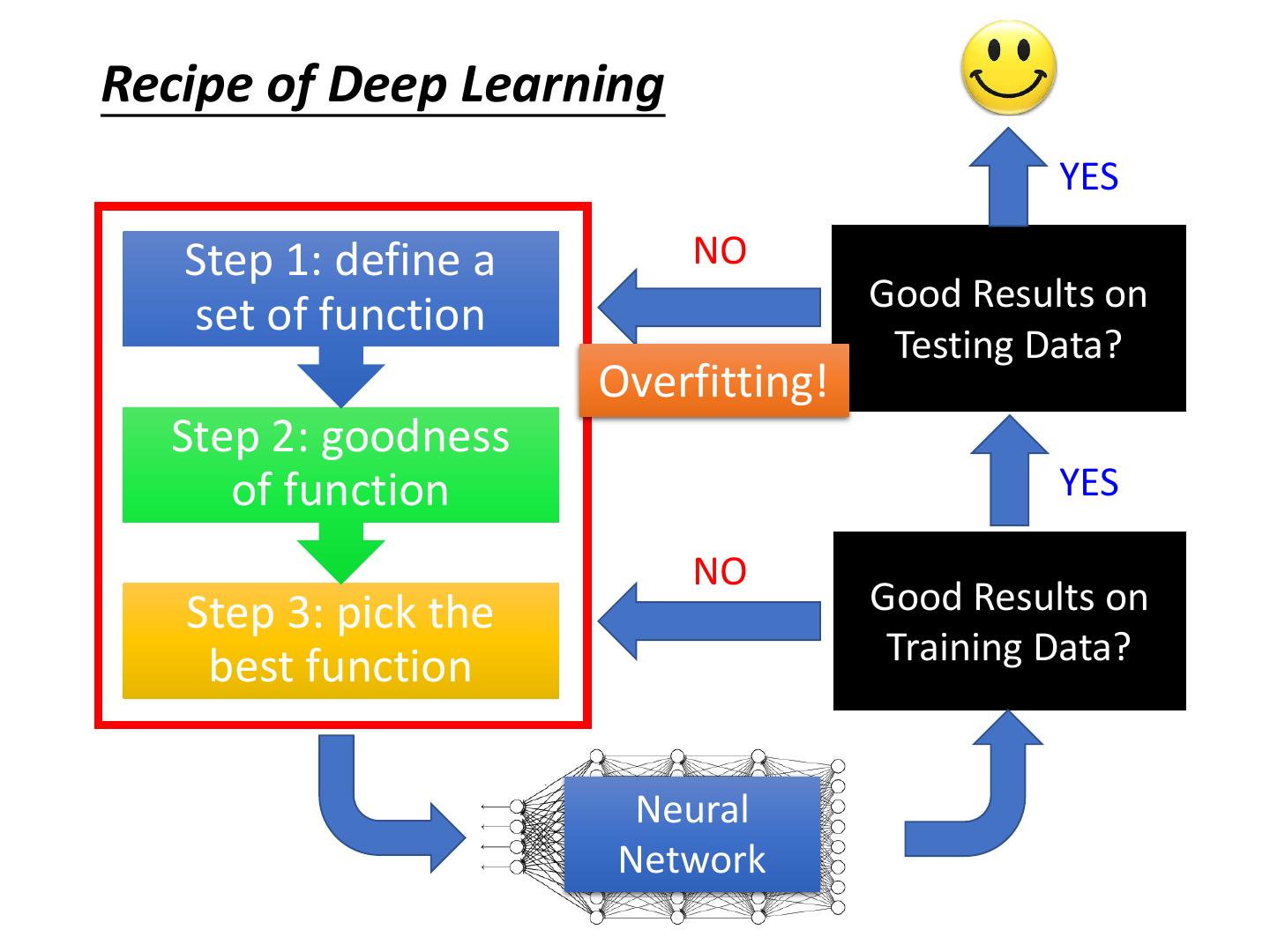
2 .Recipe of Deep Learning YES Step 1: define a NO Good Results on set of function Testing Data? Overfitting! Step 2: goodness of function YES NO Step 3: pick the Good Results on best function Training Data? Neural Network 

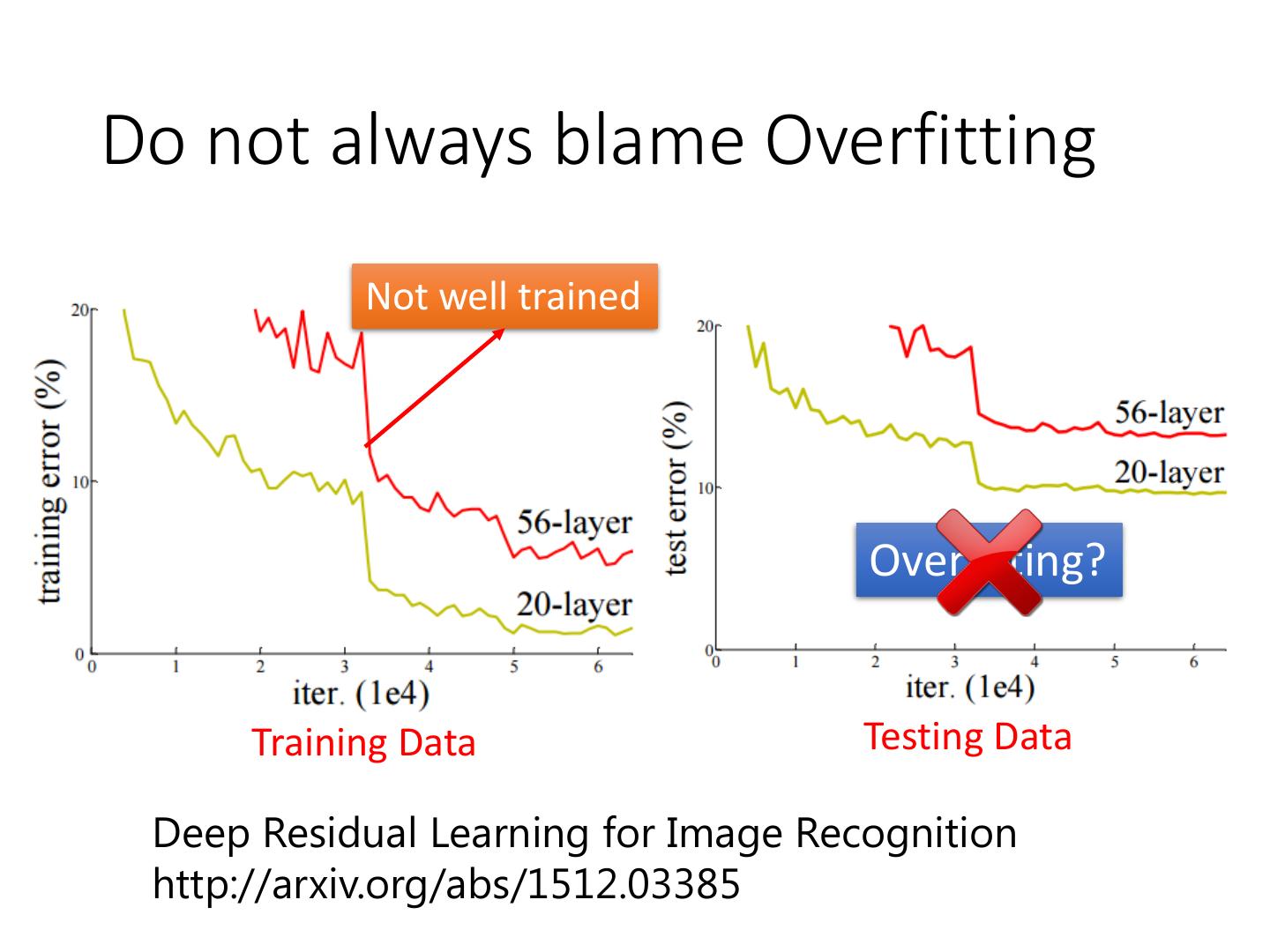
3 .Do not always blame Overfitting Not well trained Overfitting? Training Data Testing Data Deep Residual Learning for Image Recognition http://arxiv.org/abs/1512.03385 

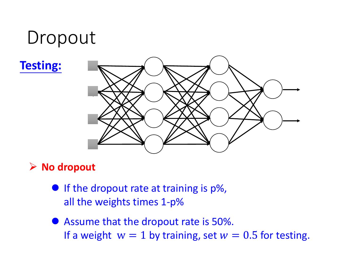
4 .Recipe of Deep Learning YES Good Results on Different approaches for Testing Data? different problems. e.g. dropout for good results YES on testing data Good Results on Training Data? Neural Network 

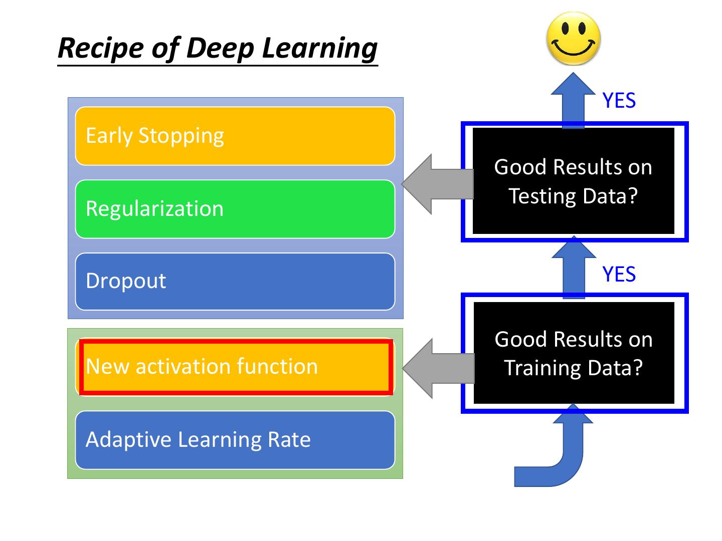
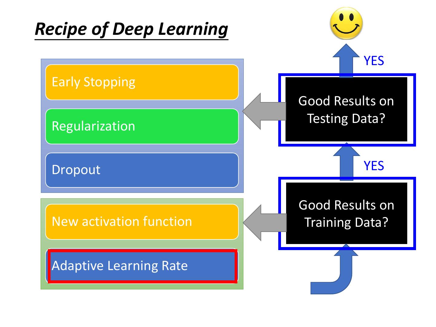
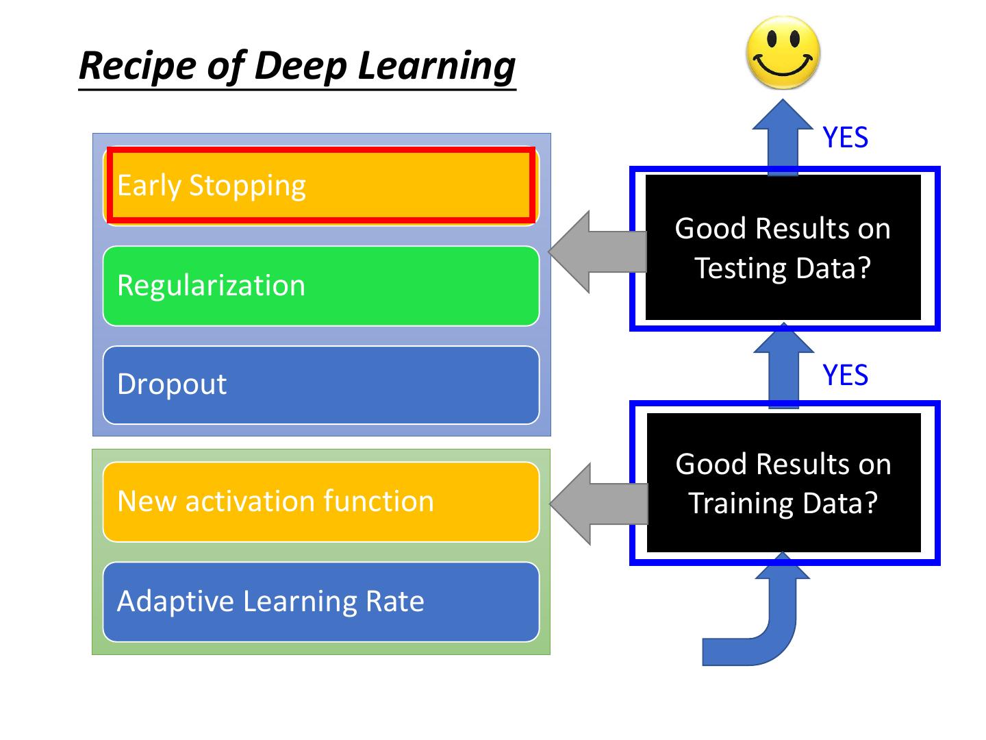
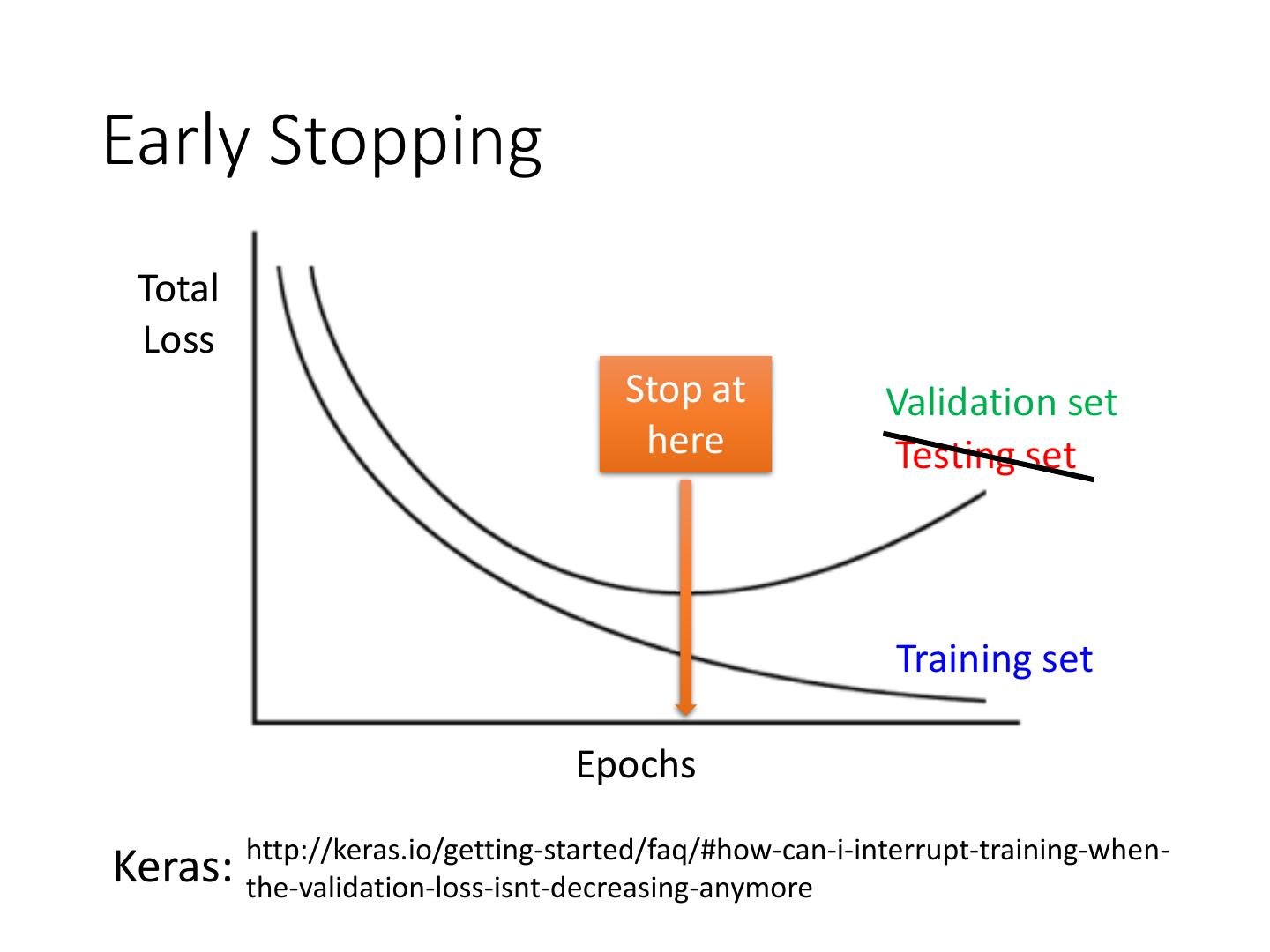
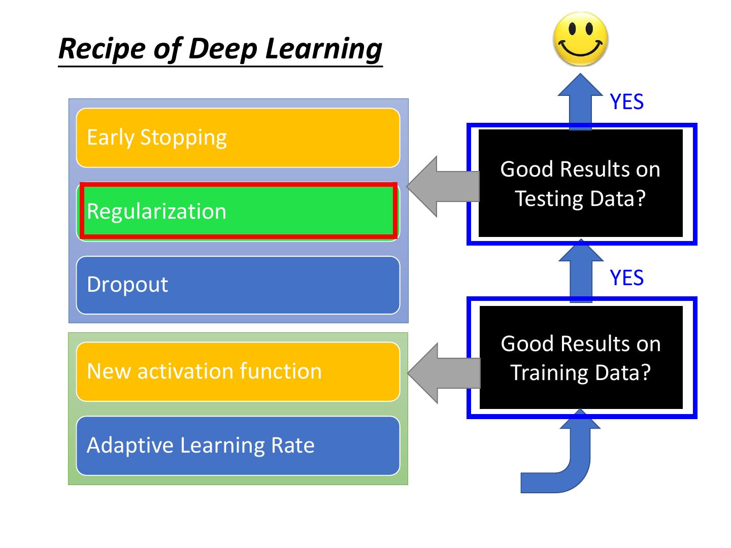
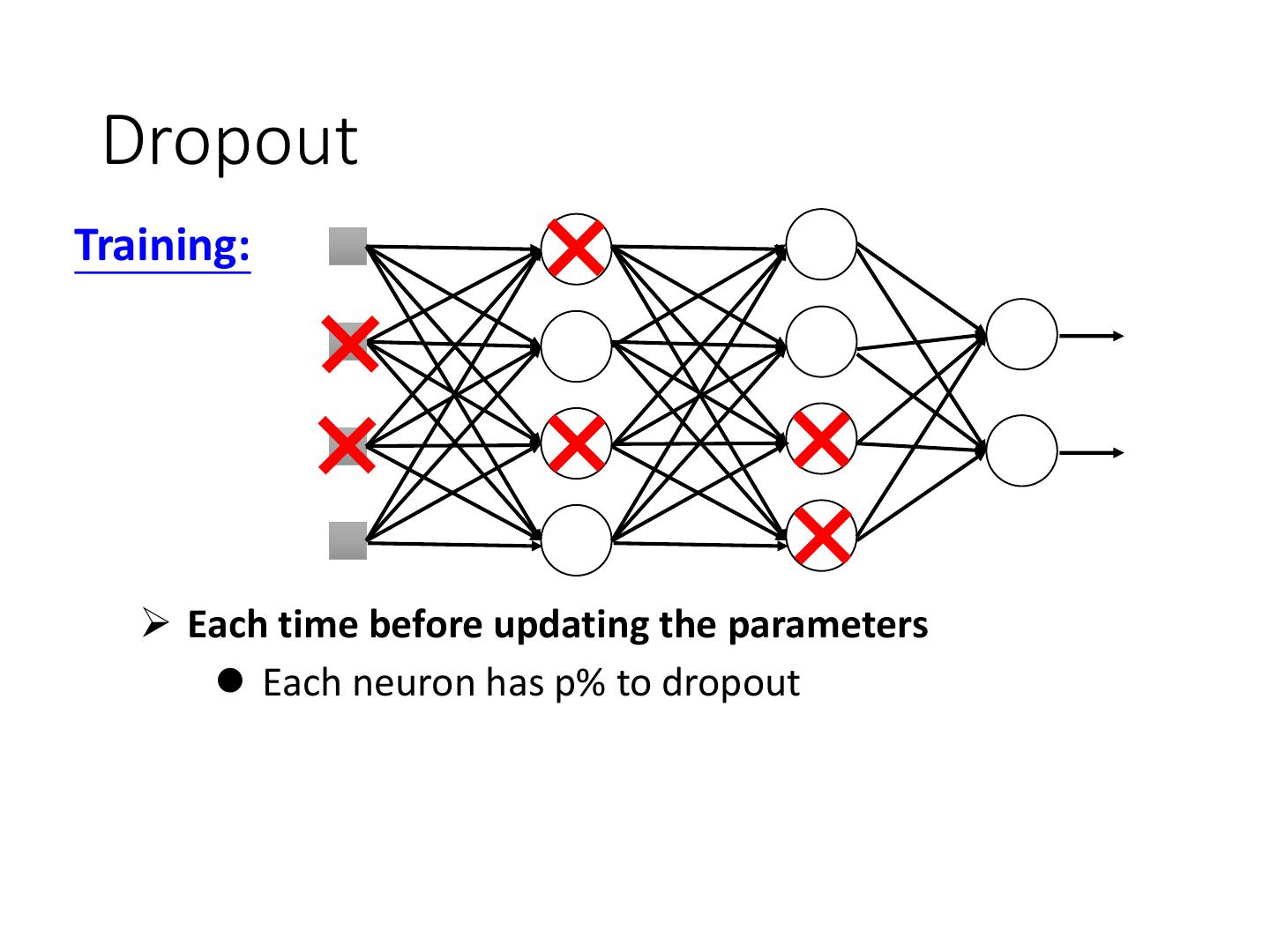
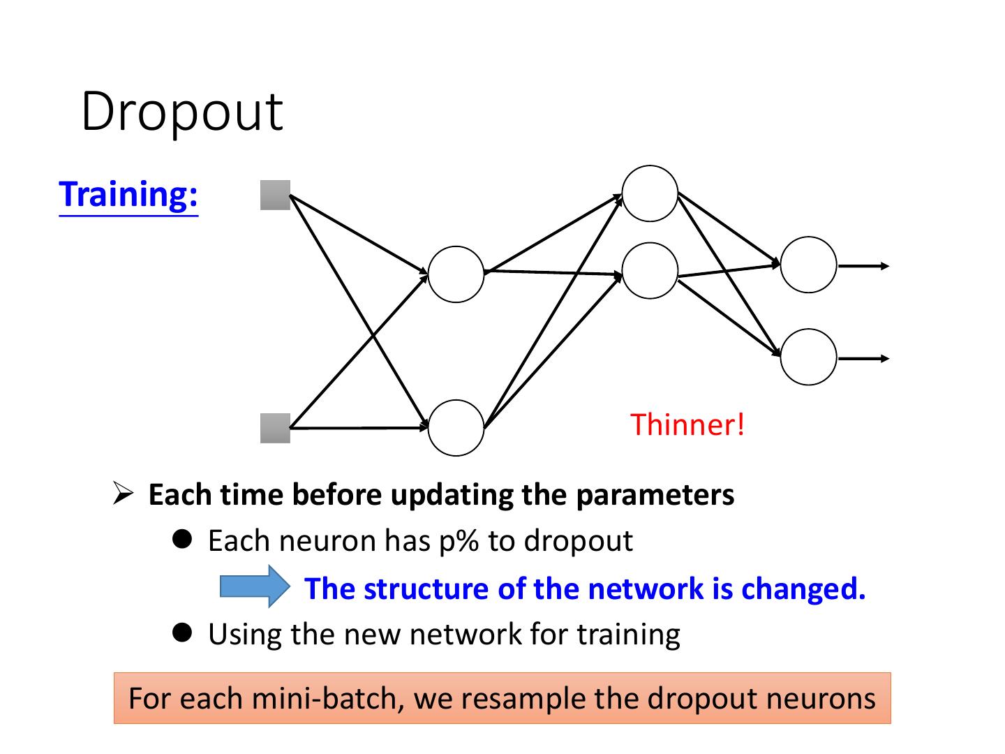
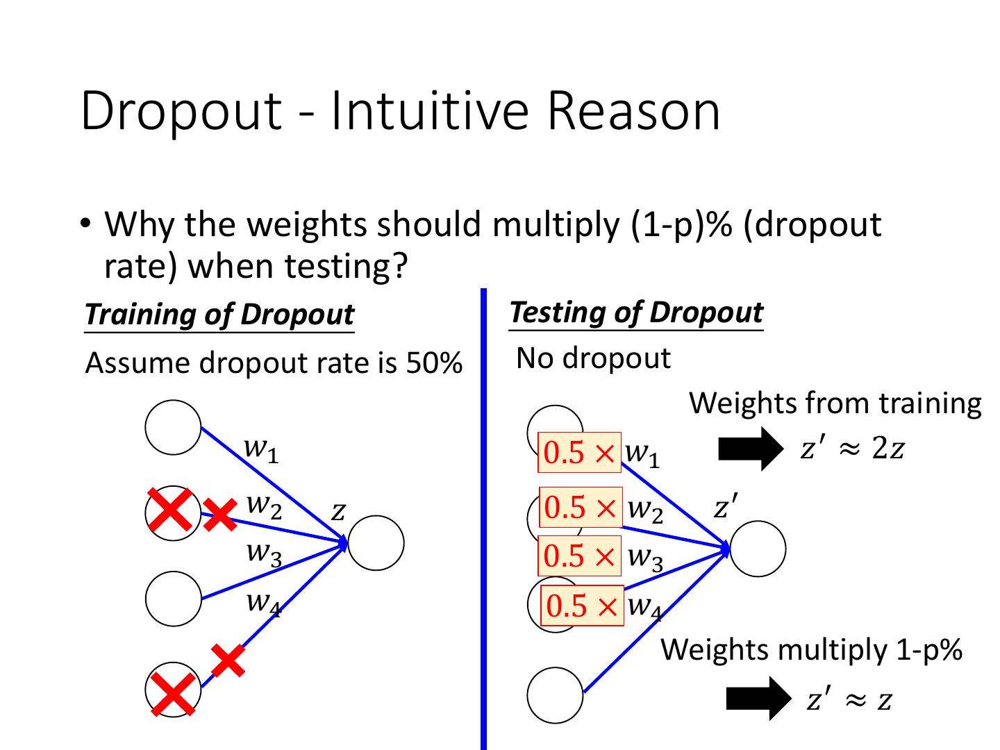
5 .Recipe of Deep Learning YES Early Stopping Good Results on Testing Data? Regularization Dropout YES Good Results on New activation function Training Data? Adaptive Learning Rate 

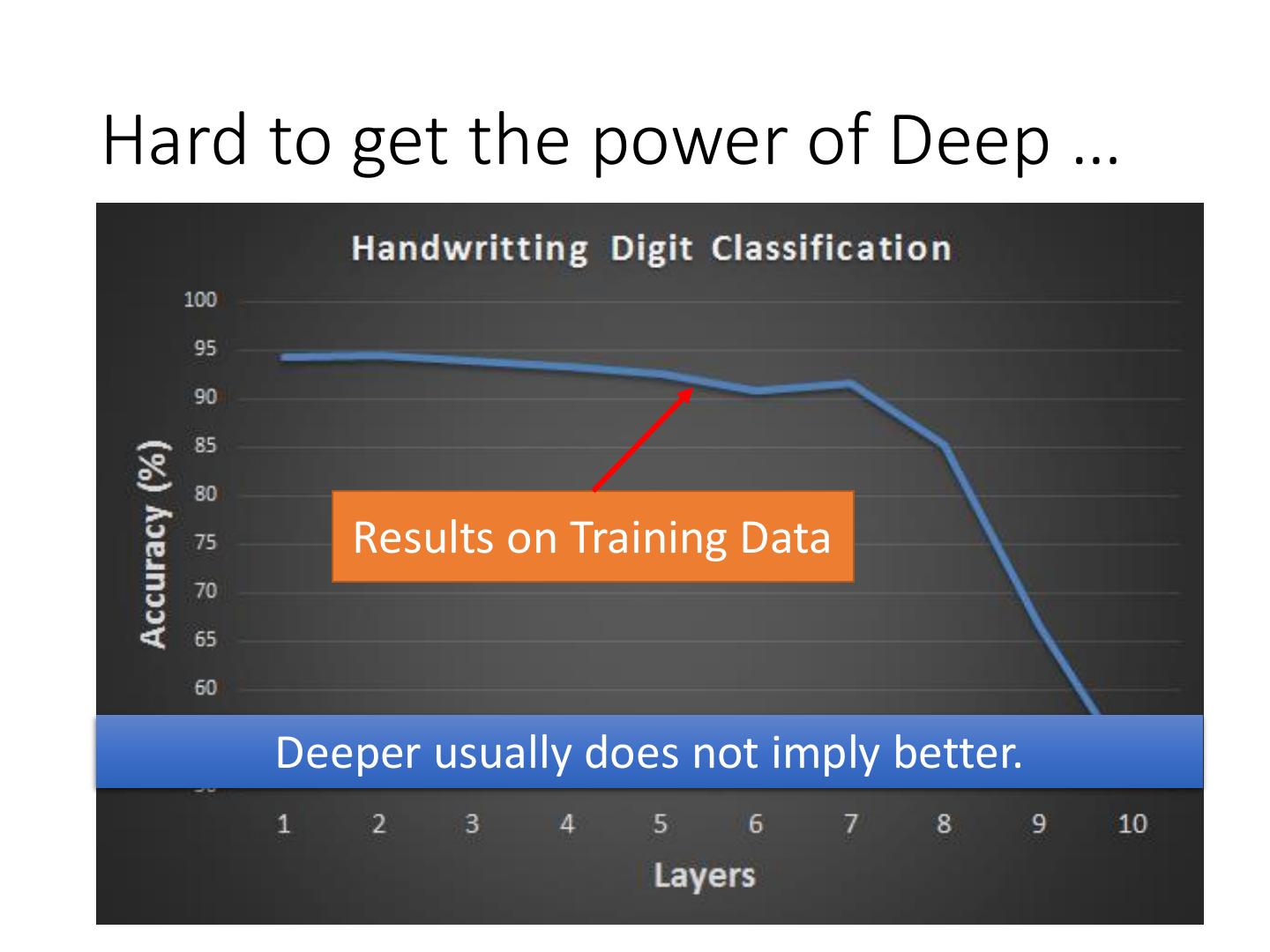
6 .Hard to get the power of Deep … Results on Training Data Deeper usually does not imply better. 

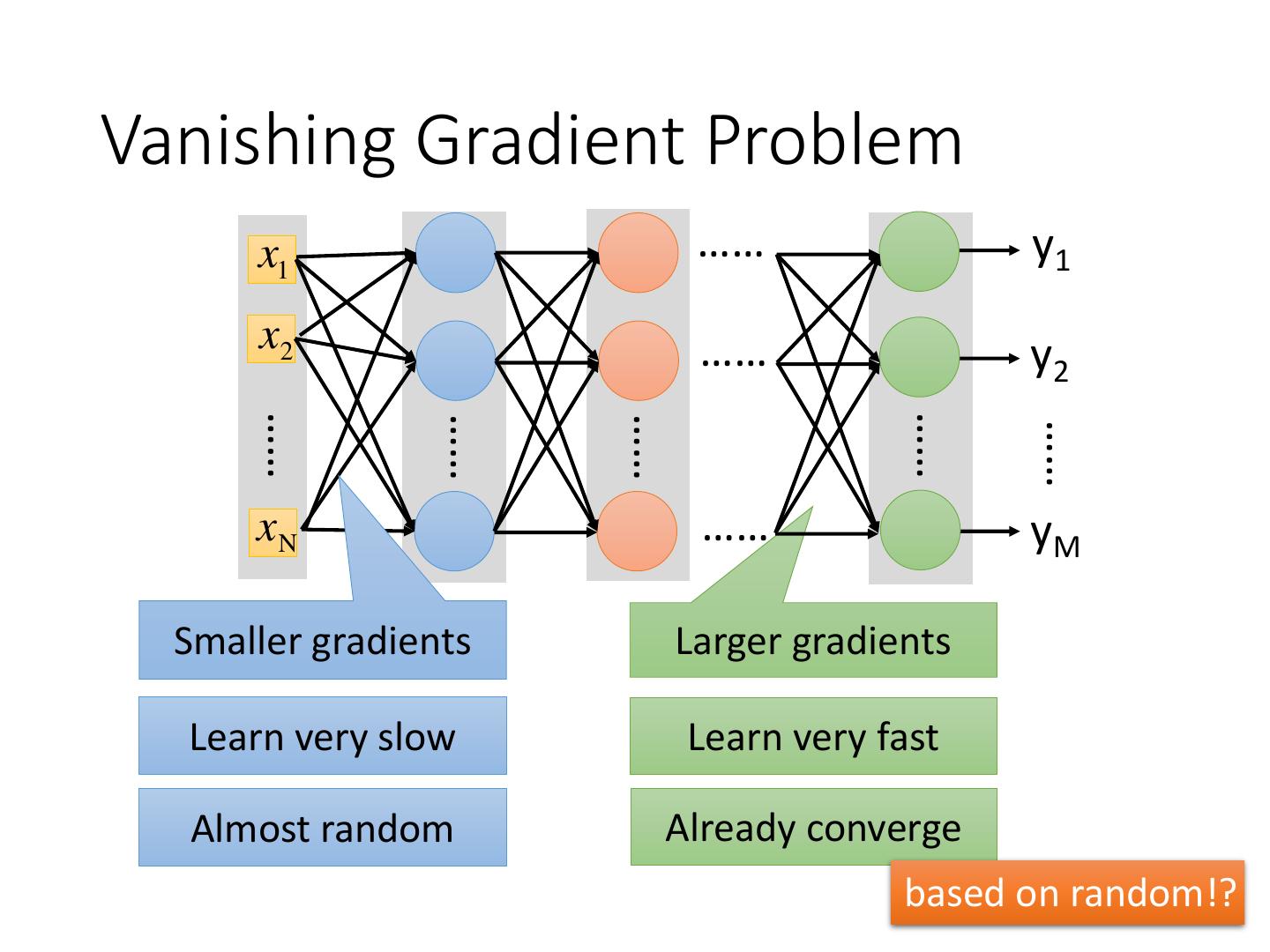
7 .Vanishing Gradient Problem x1 …… y1 x2 …… y2 …… …… …… …… …… xN …… yM Smaller gradients Larger gradients Learn very slow Learn very fast Almost random Already converge based on random!? 

8 .Vanishing Gradient Problem Smaller gradients x1 …… 𝑦1 𝑦ො1 Small x2 output …… 𝑦2 𝑦ො2 …… …… …… …… 𝑙 …… …… +∆𝑙 xN …… 𝑦𝑀 𝑦 ො Large 𝑀 +∆𝑤 input Intuitive way to compute the derivatives … 𝜕𝑙 ∆𝑙 =? 𝜕𝑤 ∆𝑤 

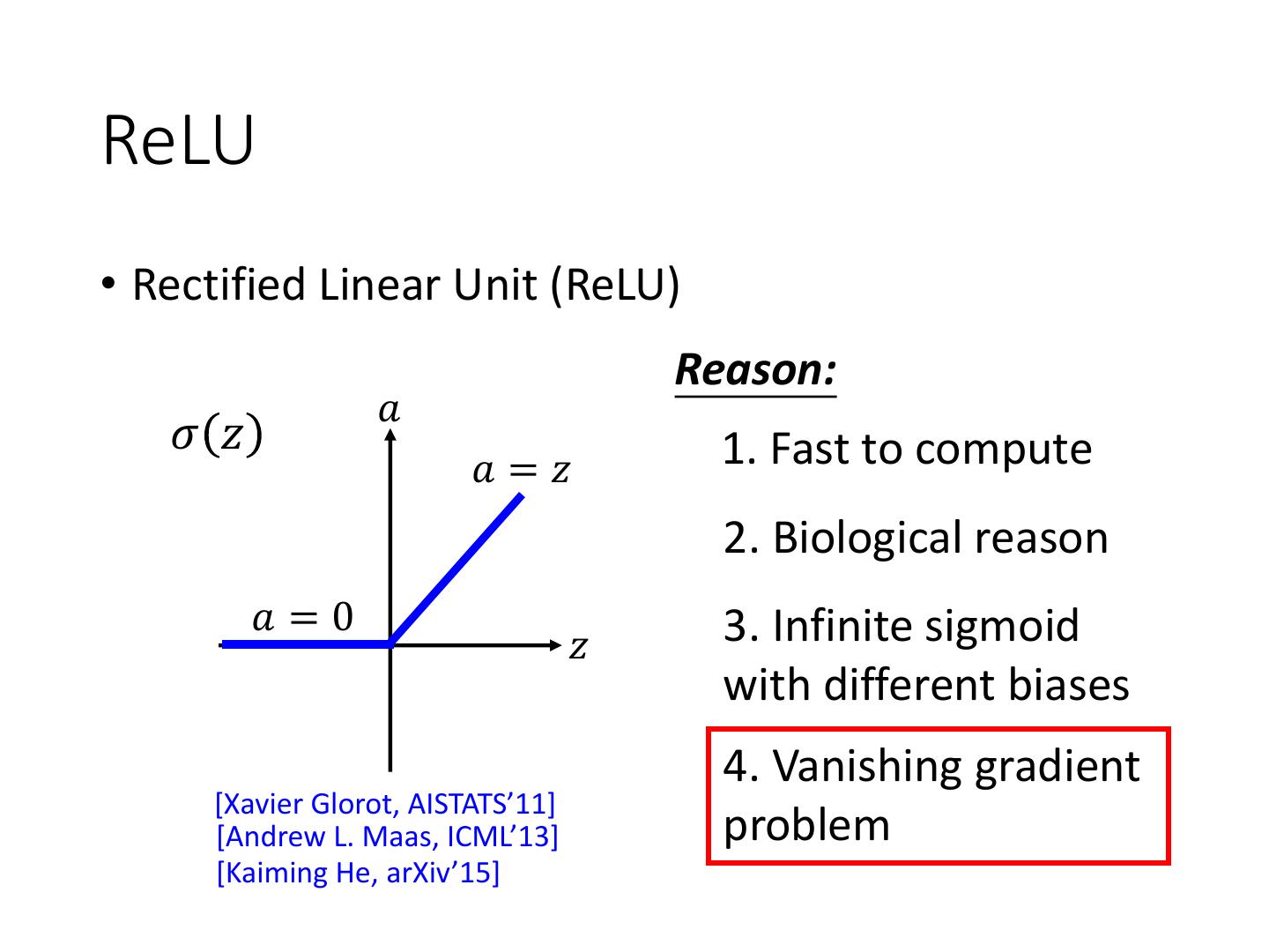
9 .ReLU • Rectified Linear Unit (ReLU) Reason: 𝑎 𝜎 𝑧 1. Fast to compute 𝑎=𝑧 2. Biological reason 𝑎=0 3. Infinite sigmoid 𝑧 with different biases 4. Vanishing gradient [Xavier Glorot, AISTATS’11] [Andrew L. Maas, ICML’13] problem [Kaiming He, arXiv’15] 

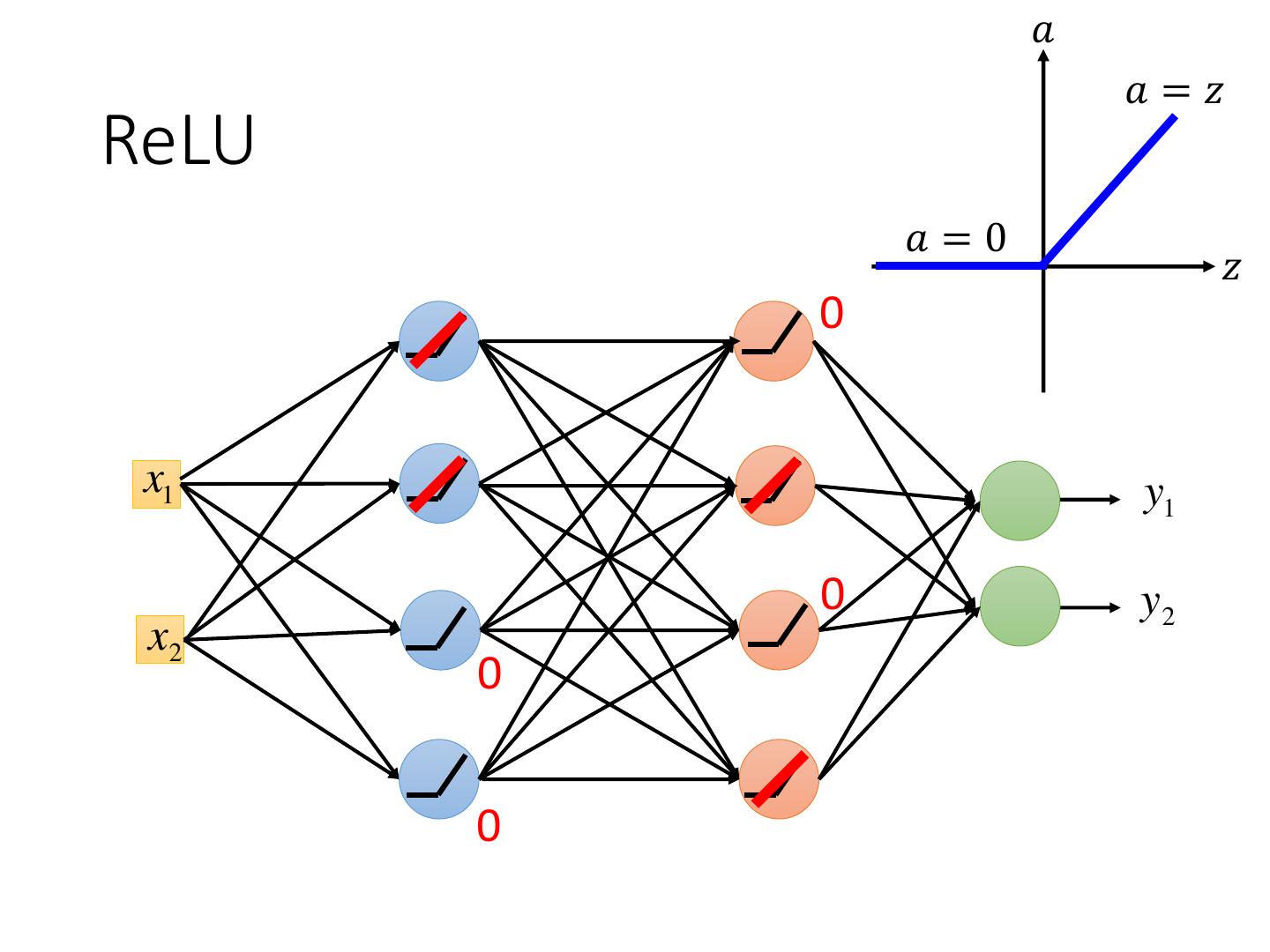
10 . 𝑎 𝑎=𝑧 ReLU 𝑎=0 𝑧 0 x1 y1 0 y2 x2 0 0 

11 . 𝑎 𝑎=𝑧 ReLU A Thinner linear network 𝑎=0 𝑧 x1 y1 y2 x2 Do not have smaller gradients 

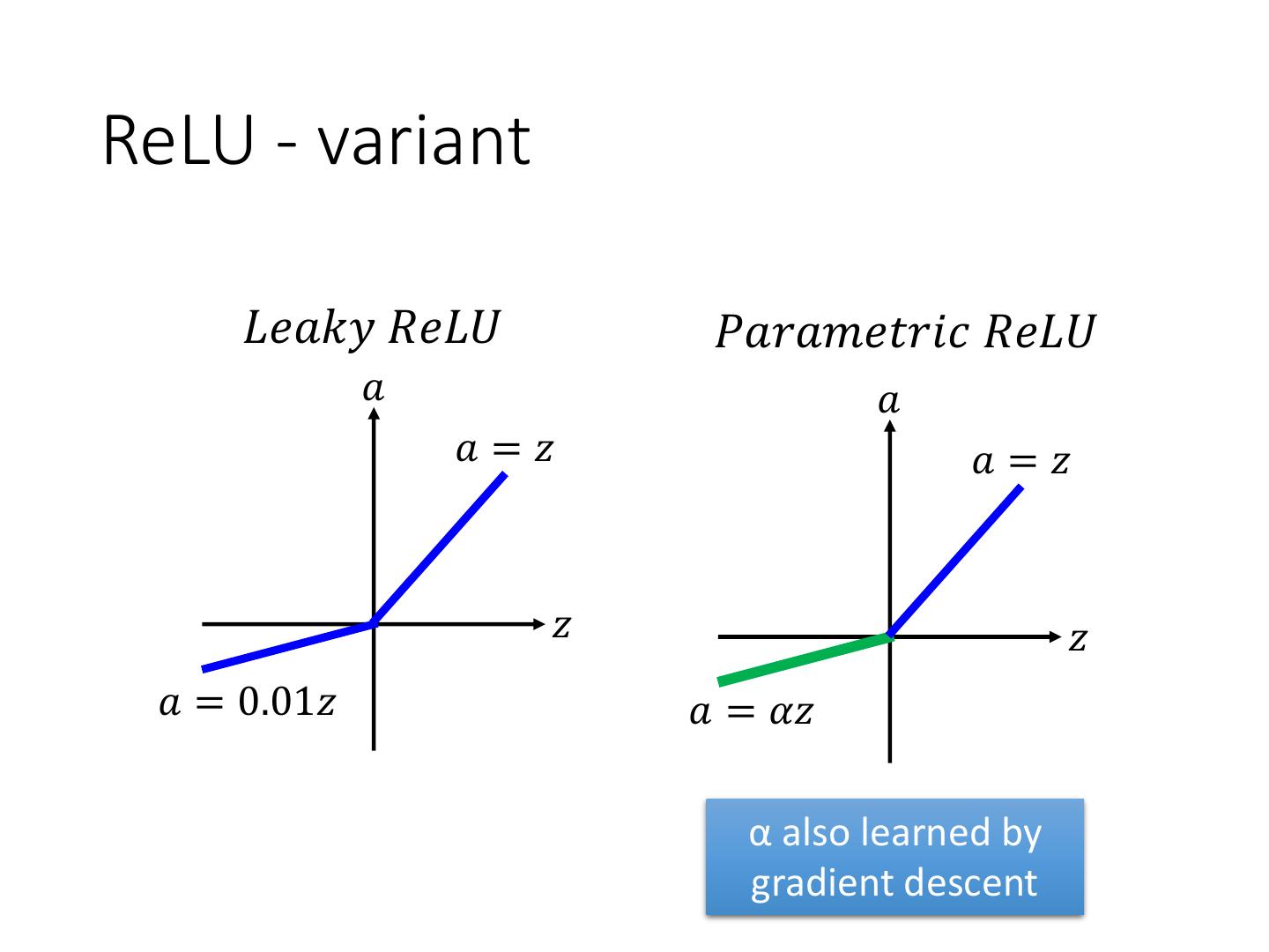
12 .ReLU - variant 𝐿𝑒𝑎𝑘𝑦 𝑅𝑒𝐿𝑈 𝑃𝑎𝑟𝑎𝑚𝑒𝑡𝑟𝑖𝑐 𝑅𝑒𝐿𝑈 𝑎 𝑎 𝑎=𝑧 𝑎=𝑧 𝑧 𝑧 𝑎 = 0.01𝑧 𝑎 = 𝛼𝑧 α also learned by gradient descent 

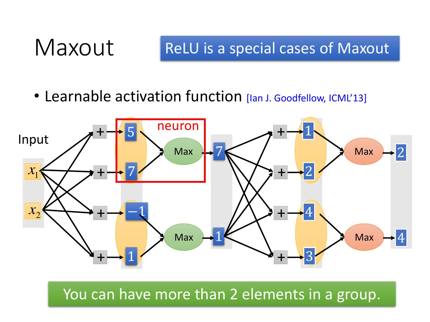
13 . Maxout ReLU is a special cases of Maxout • Learnable activation function [Ian J. Goodfellow, ICML’13] + 5 neuron + 1 Input Max 7 Max 2 x1 + 7 + 2 x2 + −1 + 4 Max 1 Max 4 + 1 + 3 You can have more than 2 elements in a group. 

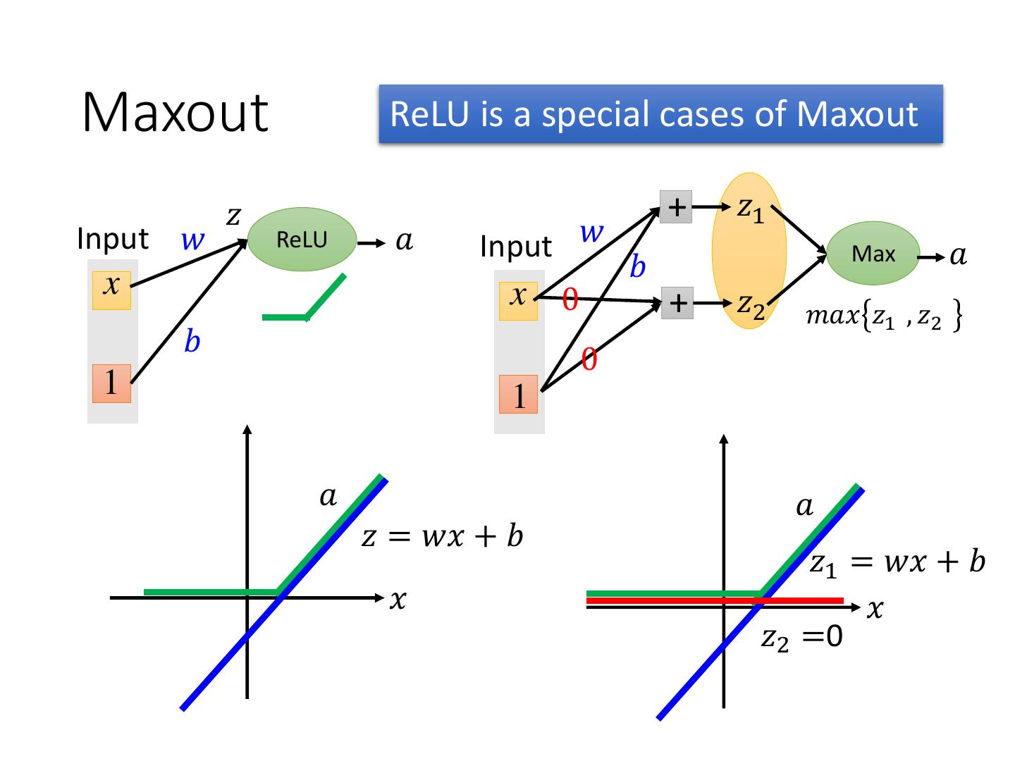
14 .Maxout ReLU is a special cases of Maxout 𝑧 + 𝑧1 Input 𝑤 ReLU 𝑎 Input 𝑤 Max 𝑎 𝑏 x x 0 + 𝑧2 𝑚𝑎𝑥 𝑧1 , 𝑧2 𝑏 0 1 1 𝑎 𝑎 𝑧 = 𝑤𝑥 + 𝑏 𝑧1 = 𝑤𝑥 + 𝑏 𝑥 𝑥 𝑧2 =0 

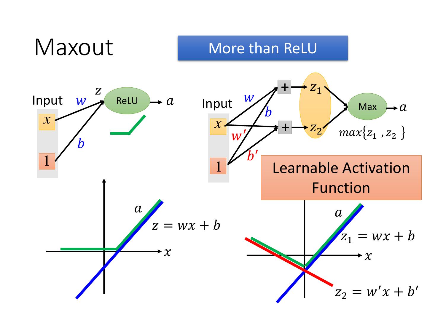
15 .Maxout More than ReLU 𝑧 + 𝑧1 Input 𝑤 ReLU 𝑎 Input 𝑤 Max 𝑎 𝑏 x x + 𝑧2 𝑚𝑎𝑥 𝑧1 , 𝑧2 𝑤′ 𝑏 1 𝑏′ 1 Learnable Activation Function 𝑎 𝑎 𝑧 = 𝑤𝑥 + 𝑏 𝑧1 = 𝑤𝑥 + 𝑏 𝑥 𝑥 𝑧2 = 𝑤 ′ 𝑥 + 𝑏 ′ 

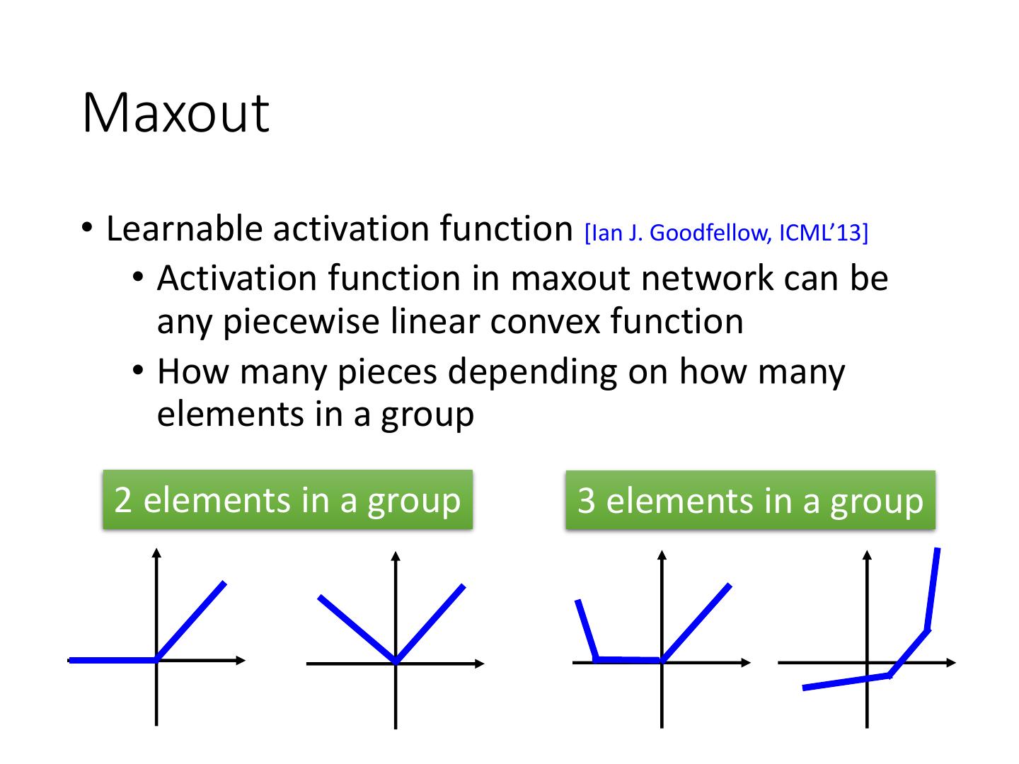
16 .Maxout • Learnable activation function [Ian J. Goodfellow, ICML’13] • Activation function in maxout network can be any piecewise linear convex function • How many pieces depending on how many elements in a group 2 elements in a group 3 elements in a group 

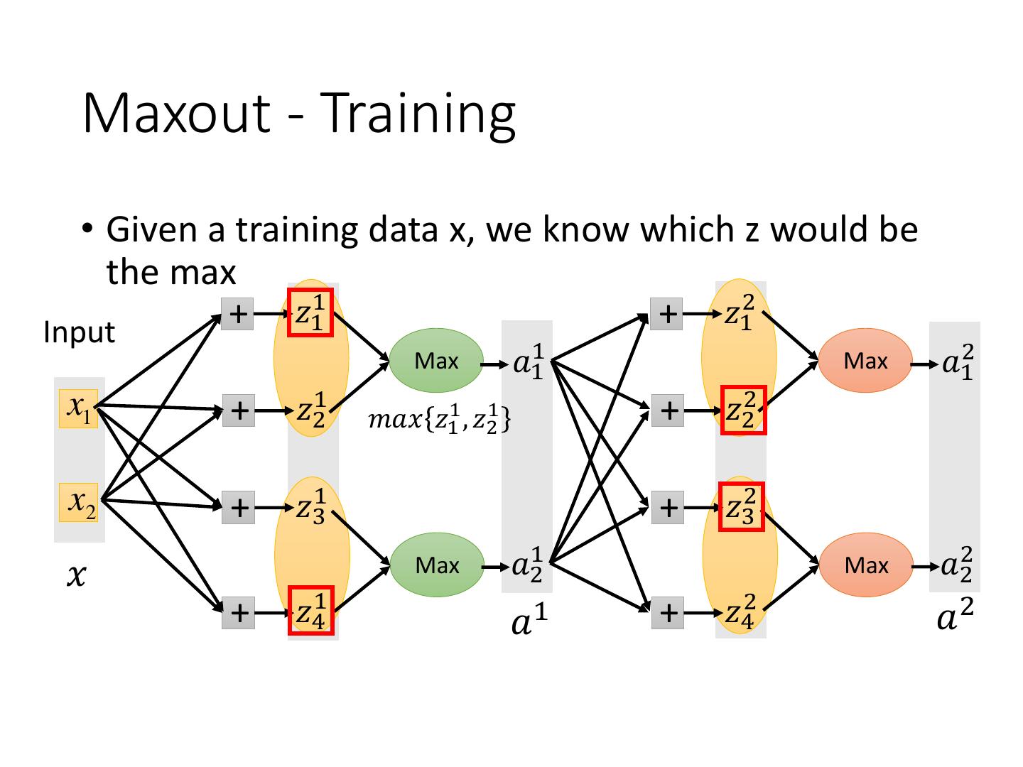
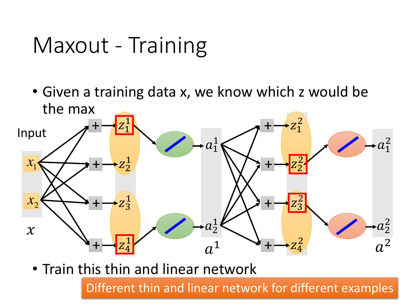
17 . Maxout - Training • Given a training data x, we know which z would be the max + 𝑧11 + 𝑧12 Input Max 𝑎11 Max 𝑎12 x1 + 𝑧21 𝑚𝑎𝑥 𝑧11 , 𝑧21 + 𝑧22 x2 + 𝑧31 + 𝑧32 𝑥 Max 𝑎21 Max 𝑎22 + 𝑧41 𝑎 1 + 𝑧42 𝑎2 

18 . Maxout - Training • Given a training data x, we know which z would be the max + 𝑧11 + 𝑧12 Input 𝑎11 𝑎12 x1 + 𝑧21 + 𝑧22 x2 + 𝑧31 + 𝑧32 𝑥 𝑎21 𝑎22 + 𝑧41 𝑎 1 + 𝑧42 𝑎2 • Train this thin and linear network Different thin and linear network for different examples 

19 .Recipe of Deep Learning YES Early Stopping Good Results on Testing Data? Regularization Dropout YES Good Results on New activation function Training Data? Adaptive Learning Rate 

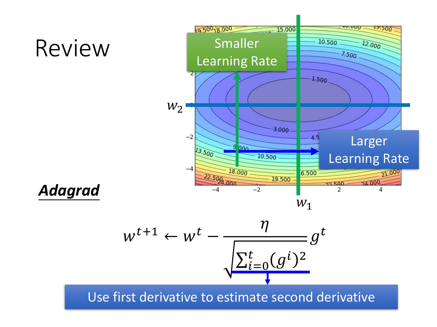
20 .Review Smaller Learning Rate 𝑤2 Larger Learning Rate Adagrad 𝑤1 𝜂 𝑤 𝑡+1 ← 𝑤𝑡 − 𝑔𝑡 σ𝑡𝑖=0 𝑔𝑖 2 Use first derivative to estimate second derivative 

21 .RMSProp Error Surface can be very complex when training NN. Smaller Learning Rate 𝑤2 Larger Learning Rate 𝑤1 

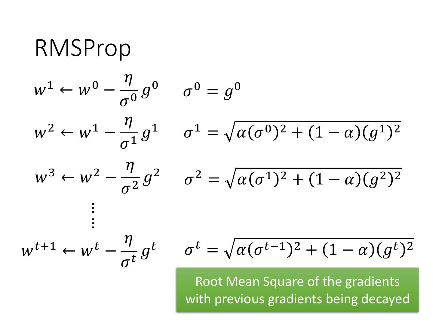
22 . RMSProp 𝜂 0 𝑤1 ← − 0𝑔𝑤0 𝜎 0 = 𝑔0 𝜎 2 1 𝜂 1 𝑤 ← 𝑤 − 1𝑔 𝜎1 = 𝛼 𝜎0 2 + 1 − 𝛼 𝑔1 2 𝜎 3 2 𝜂 2 𝑤 ← 𝑤 − 2𝑔 𝜎2 = 𝛼 𝜎1 2 + 1 − 𝛼 𝑔2 2 𝜎 …… 𝜂 𝑡 𝑤 𝑡+1 ← 𝑤𝑡 − 𝑡𝑔 𝜎𝑡 = 𝛼 𝜎 𝑡−1 2 + 1 − 𝛼 𝑔𝑡 2 𝜎 Root Mean Square of the gradients with previous gradients being decayed 

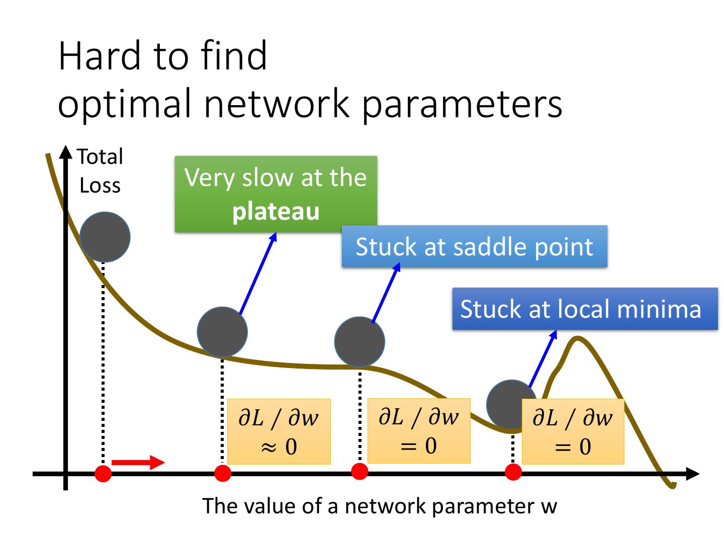
23 .Hard to find optimal network parameters Total Loss Very slow at the plateau Stuck at saddle point Stuck at local minima 𝜕𝐿 ∕ 𝜕𝑤 𝜕𝐿 ∕ 𝜕𝑤 𝜕𝐿 ∕ 𝜕𝑤 ≈0 =0 =0 The value of a network parameter w 

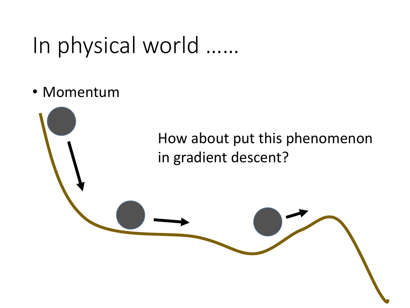
24 .In physical world …… • Momentum How about put this phenomenon in gradient descent? 

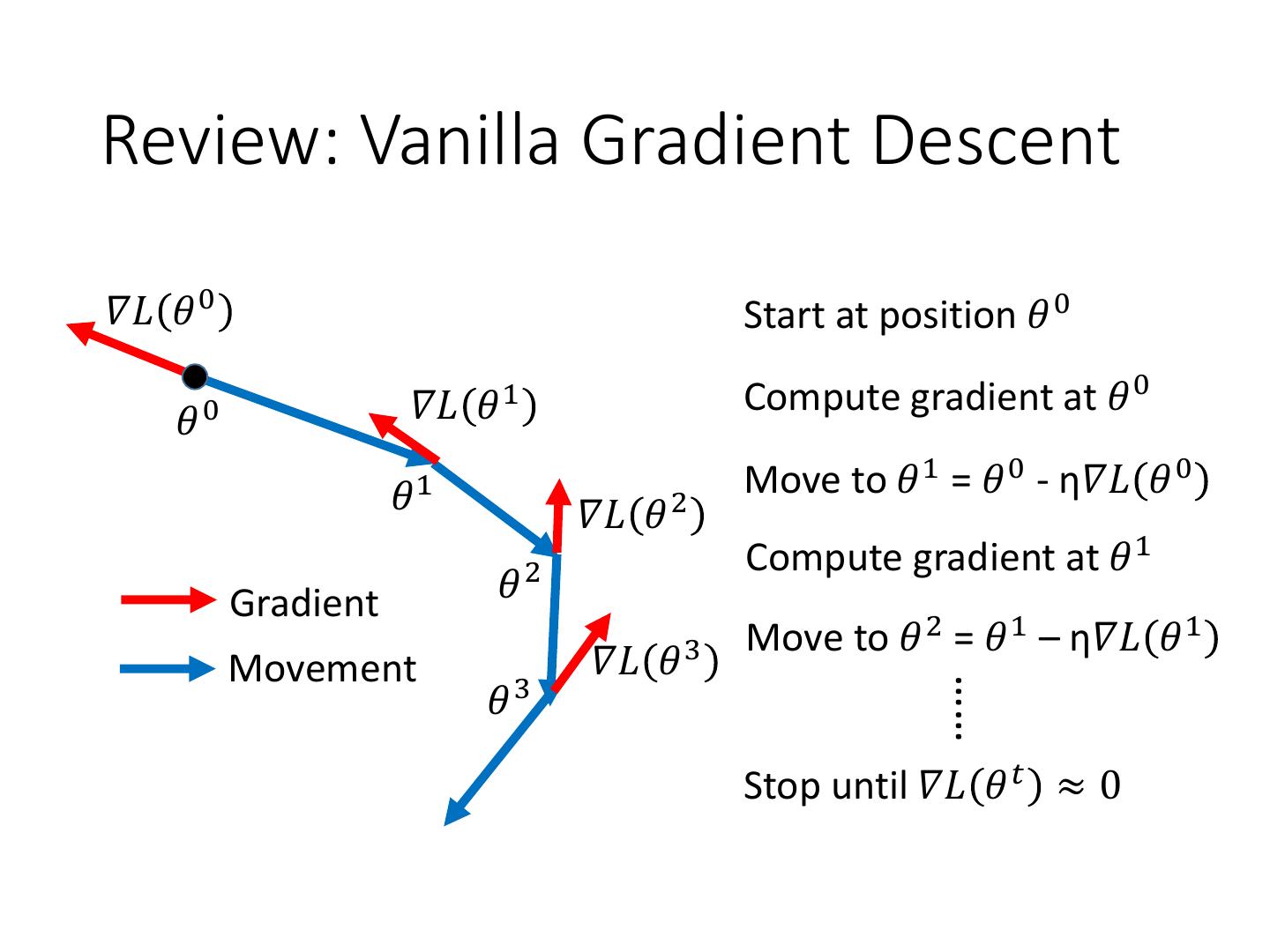
25 .Review: Vanilla Gradient Descent 𝛻𝐿 𝜃 0 Start at position 𝜃 0 𝛻𝐿 𝜃1 Compute gradient at 𝜃 0 𝜃0 𝜃 1 Move to 𝜃 1 = 𝜃 0 - η𝛻𝐿 𝜃 0 𝛻𝐿 𝜃 2 Compute gradient at 𝜃 1 Gradient 𝜃2 Move to 𝜃 2 = 𝜃 1 – η𝛻𝐿 𝜃 1 Movement 𝛻𝐿 𝜃3 𝜃3 …… Stop until 𝛻𝐿 𝜃 𝑡 ≈ 0 

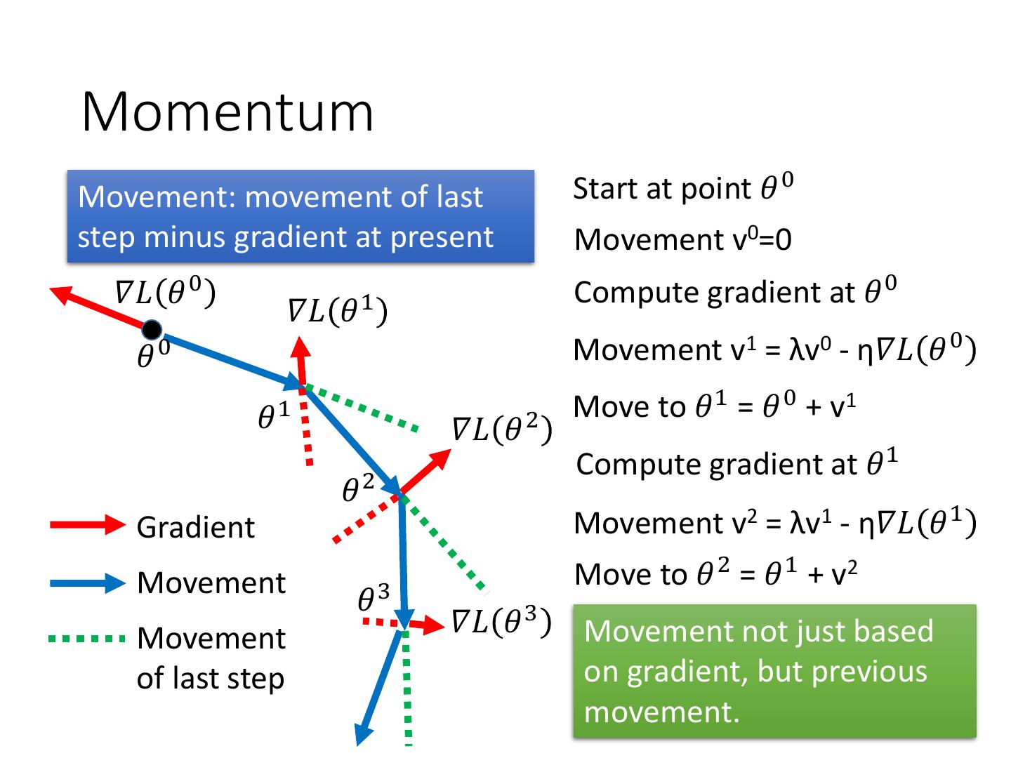
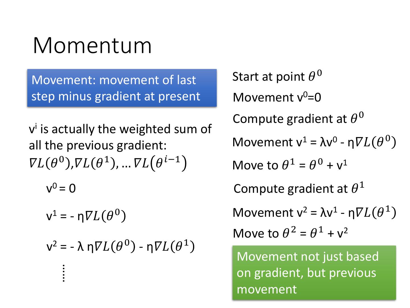
26 .Momentum Movement: movement of last Start at point 𝜃 0 step minus gradient at present Movement v0=0 𝛻𝐿 𝜃 0 Compute gradient at 𝜃 0 𝛻𝐿 𝜃 1 𝜃0 Movement v1 = λv0 - η𝛻𝐿 𝜃 0 𝜃1 Move to 𝜃 1 = 𝜃 0 + v1 𝛻𝐿 𝜃 2 Compute gradient at 𝜃 1 𝜃2 Gradient Movement v2 = λv1 - η𝛻𝐿 𝜃 1 Movement Move to 𝜃 2 = 𝜃 1 + v2 𝜃3 Movement 𝛻𝐿 𝜃 3 Movement not just based of last step on gradient, but previous movement. 

27 .Momentum Movement: movement of last Start at point 𝜃 0 step minus gradient at present Movement v0=0 Compute gradient at 𝜃 0 vi is actually the weighted sum of all the previous gradient: Movement v1 = λv0 - η𝛻𝐿 𝜃 0 𝛻𝐿 𝜃 0 ,𝛻𝐿 𝜃 1 , … 𝛻𝐿 𝜃 𝑖−1 Move to 𝜃 1 = 𝜃 0 + v1 v0 = 0 Compute gradient at 𝜃 1 v1 = - η𝛻𝐿 𝜃0 Movement v2 = λv1 - η𝛻𝐿 𝜃 1 Move to 𝜃 2 = 𝜃 1 + v2 v2 = - λ η𝛻𝐿 𝜃 0 - η𝛻𝐿 𝜃 1 Movement not just based …… on gradient, but previous movement 

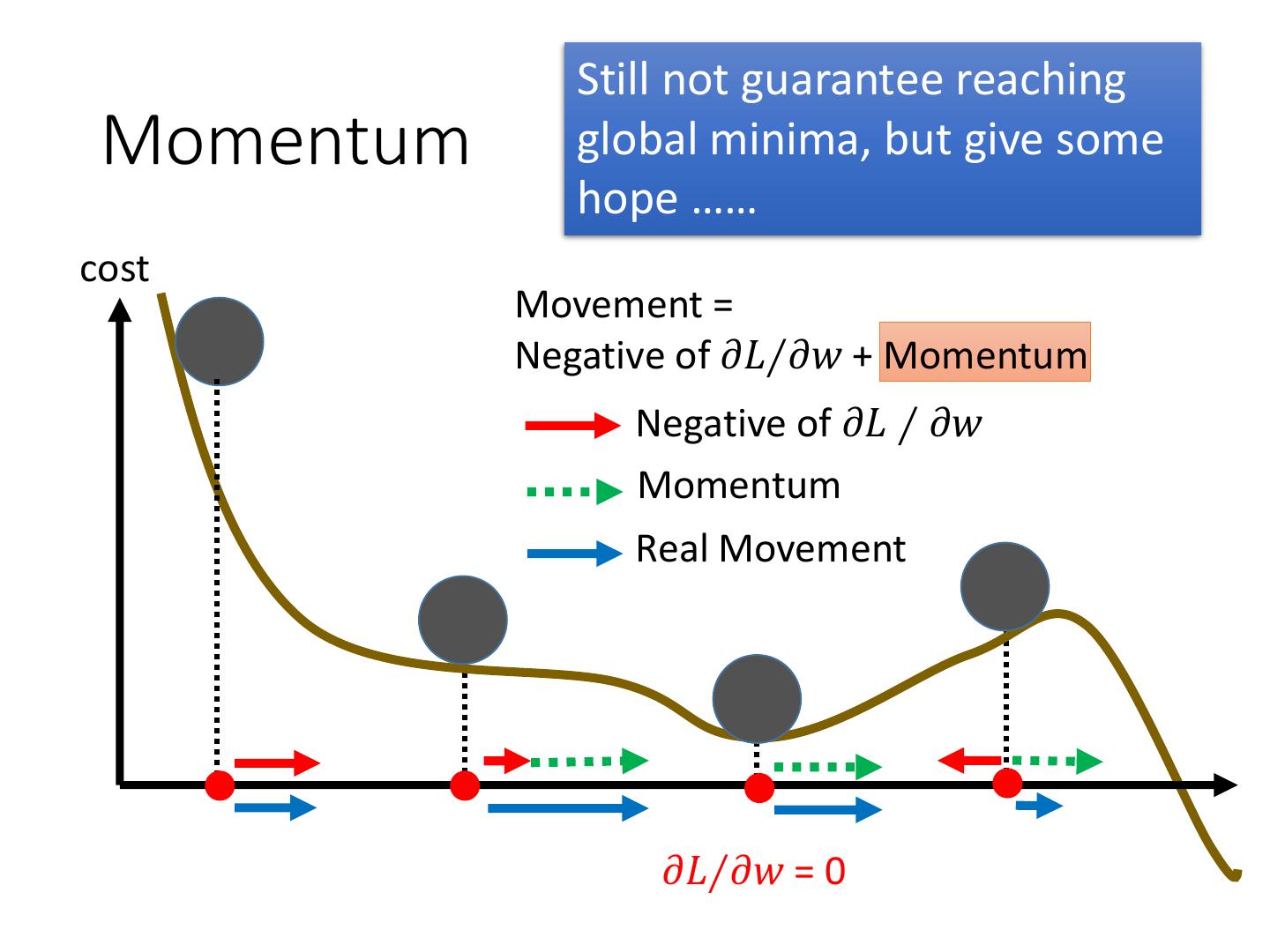
28 . Still not guarantee reaching Momentum global minima, but give some hope …… cost Movement = Negative of 𝜕𝐿∕𝜕𝑤 + Momentum Negative of 𝜕𝐿 ∕ 𝜕𝑤 Momentum Real Movement 𝜕𝐿∕𝜕𝑤 = 0 

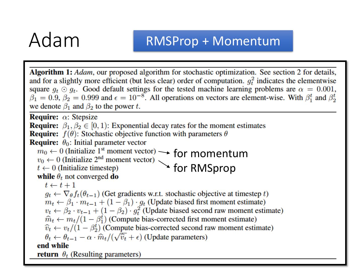
29 .Adam RMSProp + Momentum for momentum for RMSprop