Semi-supervised Learning

1 .Semi-supervised Learning 

2 .Introduction Labelled data cat dog Unlabeled data (Image of cats and dogs without labeling) 

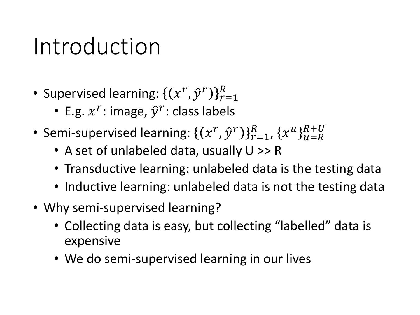
3 .Introduction • Supervised learning: 𝑥 𝑟 , 𝑦ො 𝑟 𝑅𝑟=1 • E.g. 𝑥 𝑟 : image, 𝑦ො 𝑟 : class labels • Semi-supervised learning: 𝑥 𝑟 , 𝑦ො 𝑟 𝑅𝑟=1 , 𝑥 𝑢 𝑅+𝑈 𝑢=𝑅 • A set of unlabeled data, usually U >> R • Transductive learning: unlabeled data is the testing data • Inductive learning: unlabeled data is not the testing data • Why semi-supervised learning? • Collecting data is easy, but collecting “labelled” data is expensive • We do semi-supervised learning in our lives 

4 .Why semi-supervised learning helps? Who knows? The distribution of the unlabeled data tell us something. Usually with some assumptions 

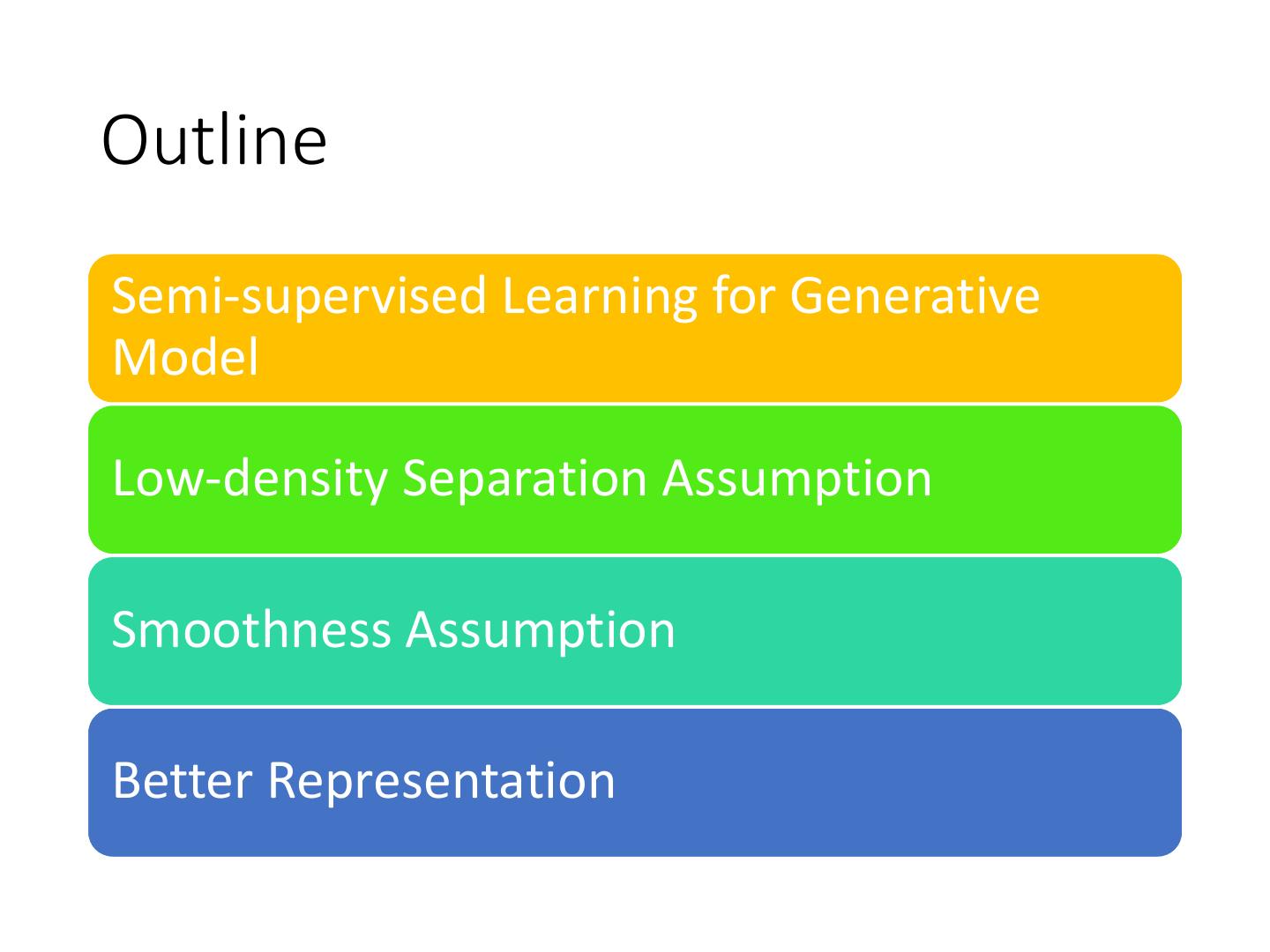
5 .Outline Semi-supervised Learning for Generative Model Low-density Separation Assumption Smoothness Assumption Better Representation 

6 .Semi-supervised Learning for Generative Model 

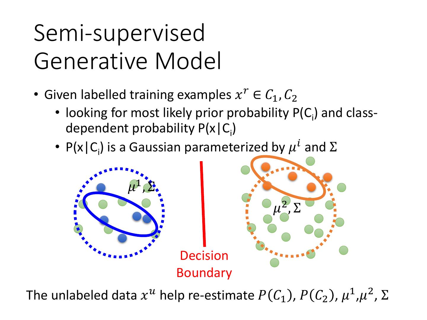
7 .Supervised Generative Model • Given labelled training examples 𝑥 𝑟 ∈ 𝐶1 , 𝐶2 • looking for most likely prior probability P(Ci) and class- dependent probability P(x|Ci) • P(x|Ci) is a Gaussian parameterized by 𝜇𝑖 and Σ 𝜇1 , Σ 𝜇2 , Σ Decision Boundary With 𝑃 𝐶1 , 𝑃 𝐶2 ,𝜇1 ,𝜇2 , Σ 𝑃 𝑥|𝐶1 𝑃 𝐶1 𝑃 𝐶1 |𝑥 = 𝑃 𝑥|𝐶1 𝑃 𝐶1 + 𝑃 𝑥|𝐶2 𝑃 𝐶2 

8 . Semi-supervised Generative Model • Given labelled training examples 𝑥 𝑟 ∈ 𝐶1 , 𝐶2 • looking for most likely prior probability P(Ci) and class- dependent probability P(x|Ci) • P(x|Ci) is a Gaussian parameterized by 𝜇𝑖 and Σ 𝜇1 , Σ 𝜇2 , Σ Decision Boundary The unlabeled data 𝑥 𝑢 help re-estimate 𝑃 𝐶1 , 𝑃 𝐶2 , 𝜇1 ,𝜇2 , Σ 

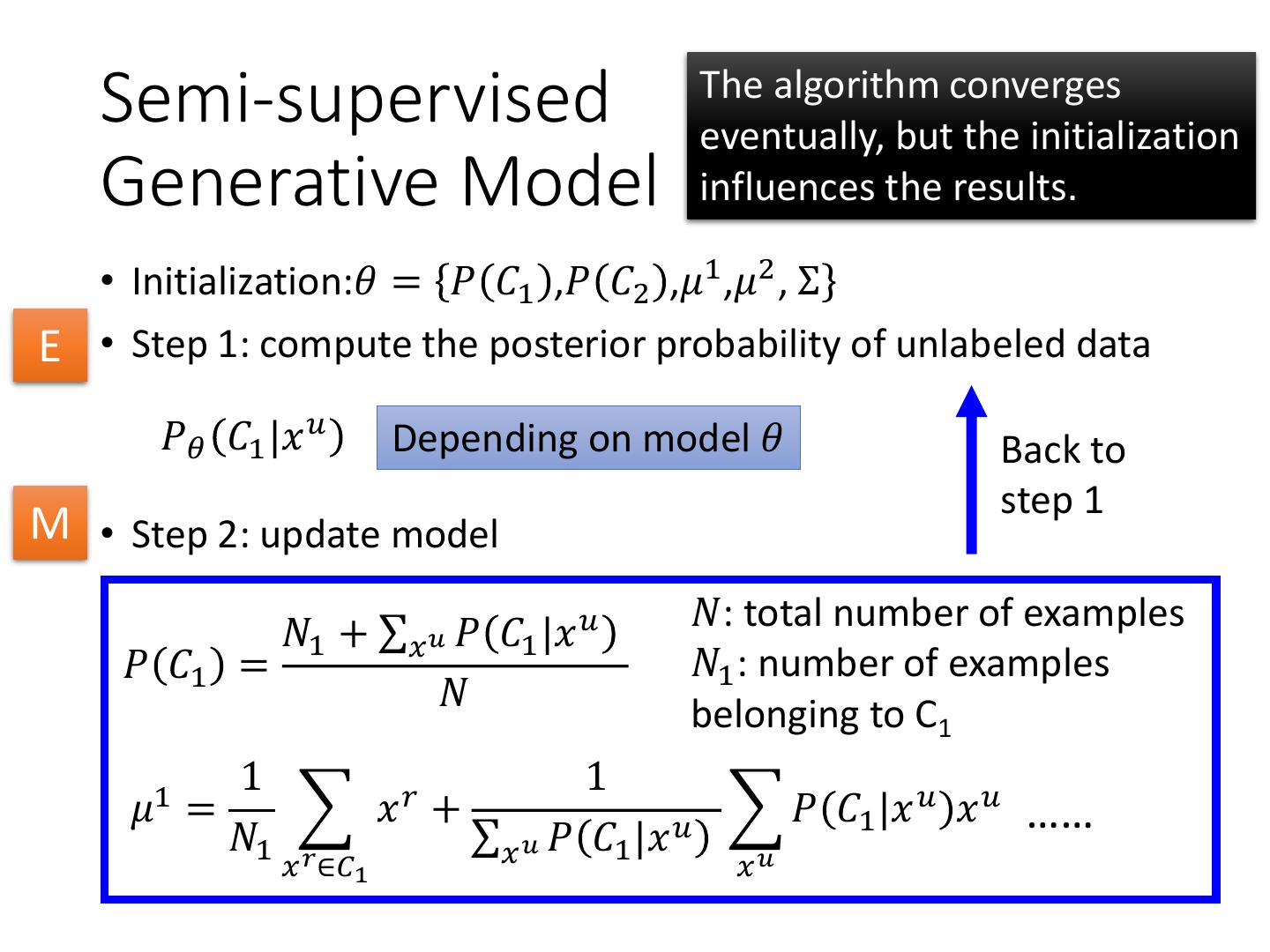
9 . Semi-supervised The algorithm converges eventually, but the initialization Generative Model influences the results. • Initialization:𝜃 = 𝑃 𝐶1 ,𝑃 𝐶2 ,𝜇1 ,𝜇2 , Σ E • Step 1: compute the posterior probability of unlabeled data 𝑃𝜃 𝐶1 |𝑥 𝑢 Depending on model 𝜃 Back to step 1 M • Step 2: update model 𝑁1 + σ𝑥 𝑢 𝑃 𝐶1 |𝑥 𝑢 𝑁: total number of examples 𝑃 𝐶1 = 𝑁1 : number of examples 𝑁 belonging to C1 1 1 𝜇1 = 𝑟 ෍ 𝑥 + ෍ 𝑃 𝐶1 |𝑥 𝑢 𝑥𝑢 …… 𝑁1 𝑟 σ𝑥 𝑢 𝑃 𝐶1 |𝑥 𝑢 𝑢 𝑥 ∈𝐶1 𝑥 

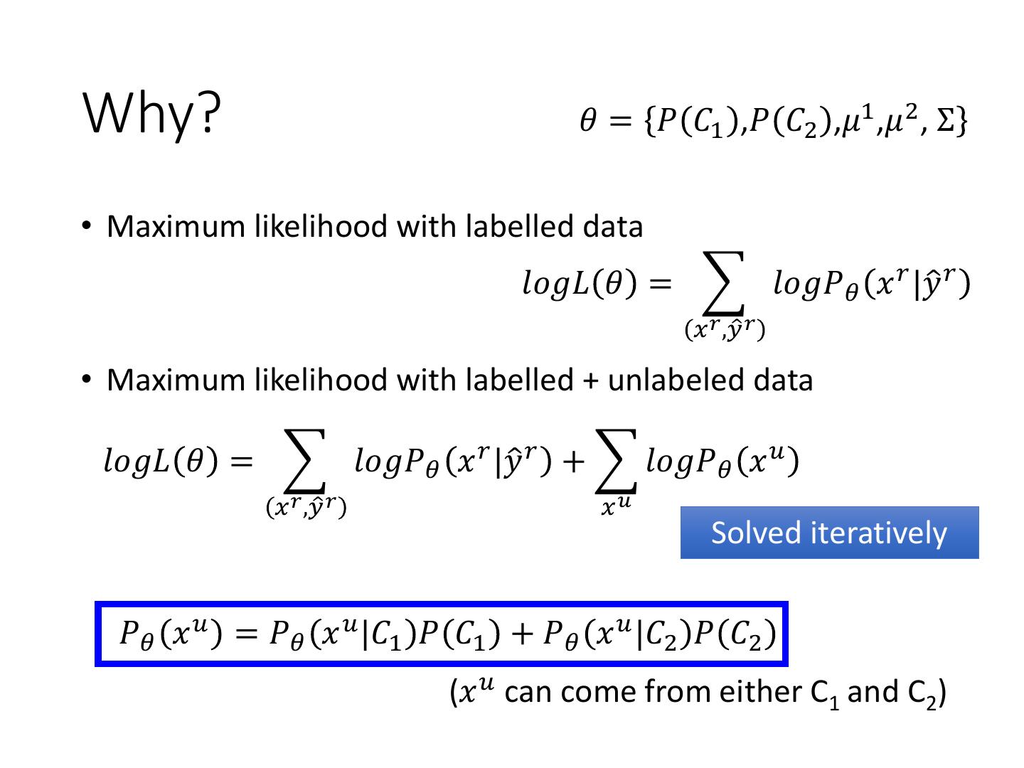
10 .Why? 𝜃 = 𝑃 𝐶1 ,𝑃 𝐶2 ,𝜇1 ,𝜇2 , Σ • Maximum likelihood with labelled data 𝑙𝑜𝑔𝐿 𝜃 = ෍ 𝑙𝑜𝑔𝑃𝜃 𝑥 𝑟 |𝑦ො 𝑟 𝑥 𝑟 ,𝑦ො 𝑟 • Maximum likelihood with labelled + unlabeled data 𝑙𝑜𝑔𝐿 𝜃 = ෍ 𝑙𝑜𝑔𝑃𝜃 𝑥 𝑟 |𝑦ො 𝑟 + ෍ 𝑙𝑜𝑔𝑃𝜃 𝑥 𝑢 𝑥 𝑟 ,𝑦ො 𝑟 𝑥𝑢 Solved iteratively 𝑃𝜃 𝑥 𝑢 = 𝑃𝜃 𝑥 𝑢 |𝐶1 𝑃 𝐶1 + 𝑃𝜃 𝑥 𝑢 |𝐶2 𝑃 𝐶2 (𝑥 𝑢 can come from either C1 and C2) 

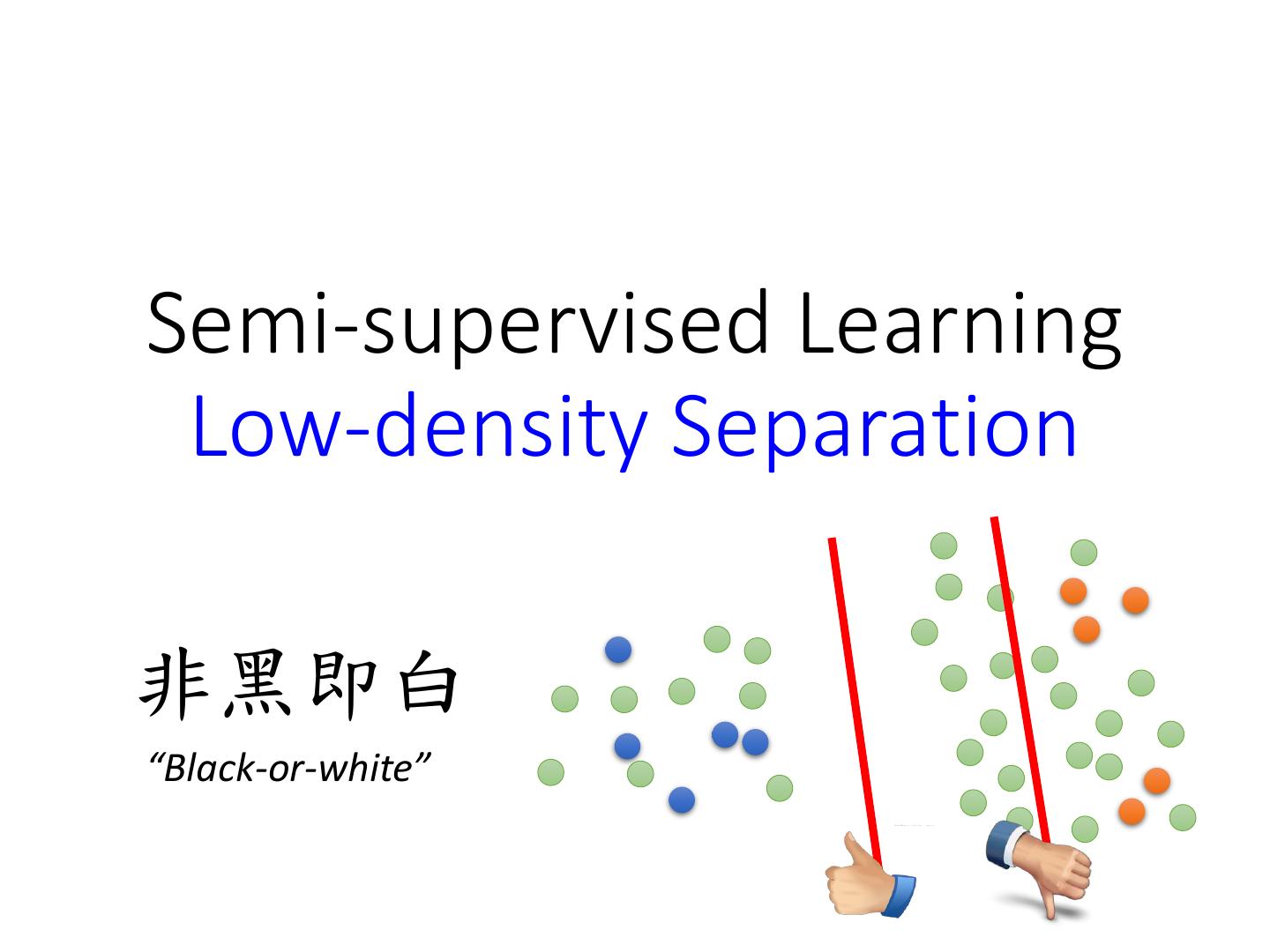
11 .Semi-supervised Learning Low-density Separation 非黑即白 “Black-or-white” 

12 .Self-training • Given: labelled data set = 𝑥 𝑟 , 𝑦ො 𝑟 𝑅𝑟=1 , unlabeled data set = 𝑥𝑢 𝑈 𝑢=1 • Repeat: • Train model 𝑓 ∗ from labelled data set You can use any model here. Regression? • Apply 𝑓 ∗ to the unlabeled data set • Obtain 𝑥 𝑢 , 𝑦 𝑢 𝑈𝑢=1 Pseudo-label • Remove a set of data from unlabeled data set, and add them into the labeled data set How to choose the data You can also provide a set remains open weight to each data. 

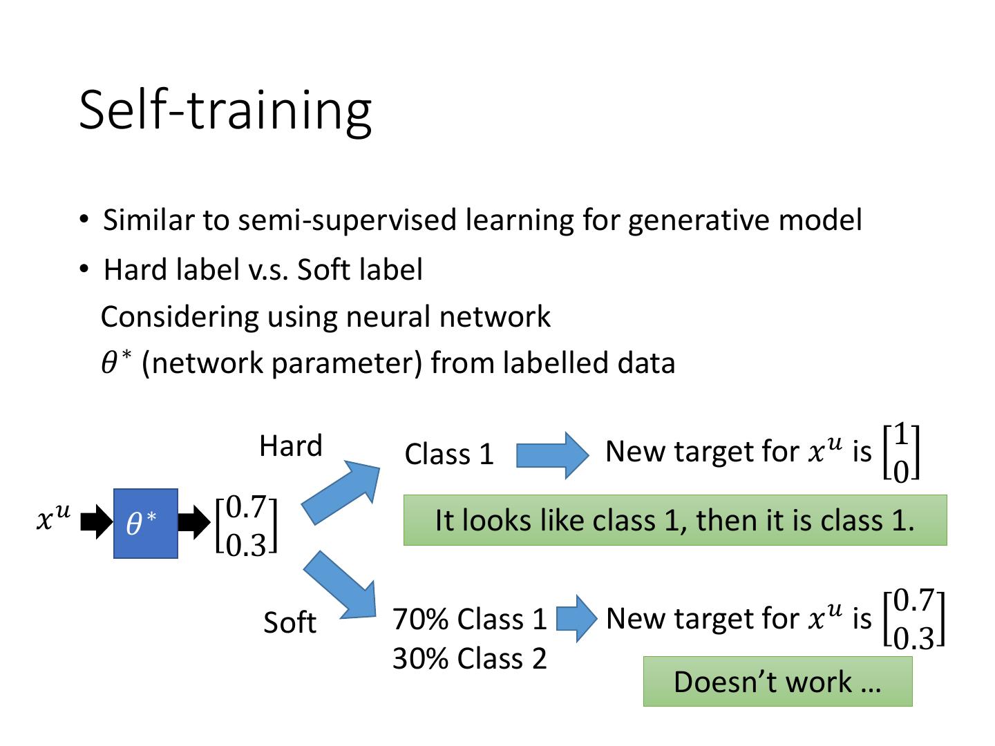
13 . Self-training • Similar to semi-supervised learning for generative model • Hard label v.s. Soft label Considering using neural network 𝜃 ∗ (network parameter) from labelled data 1 Hard Class 1 New target for 𝑥 𝑢 is 0 𝑥𝑢 0.7 𝜃∗ It looks like class 1, then it is class 1. 0.3 0.7 Soft 70% Class 1 New target for 𝑥 𝑢 is 0.3 30% Class 2 Doesn’t work … 

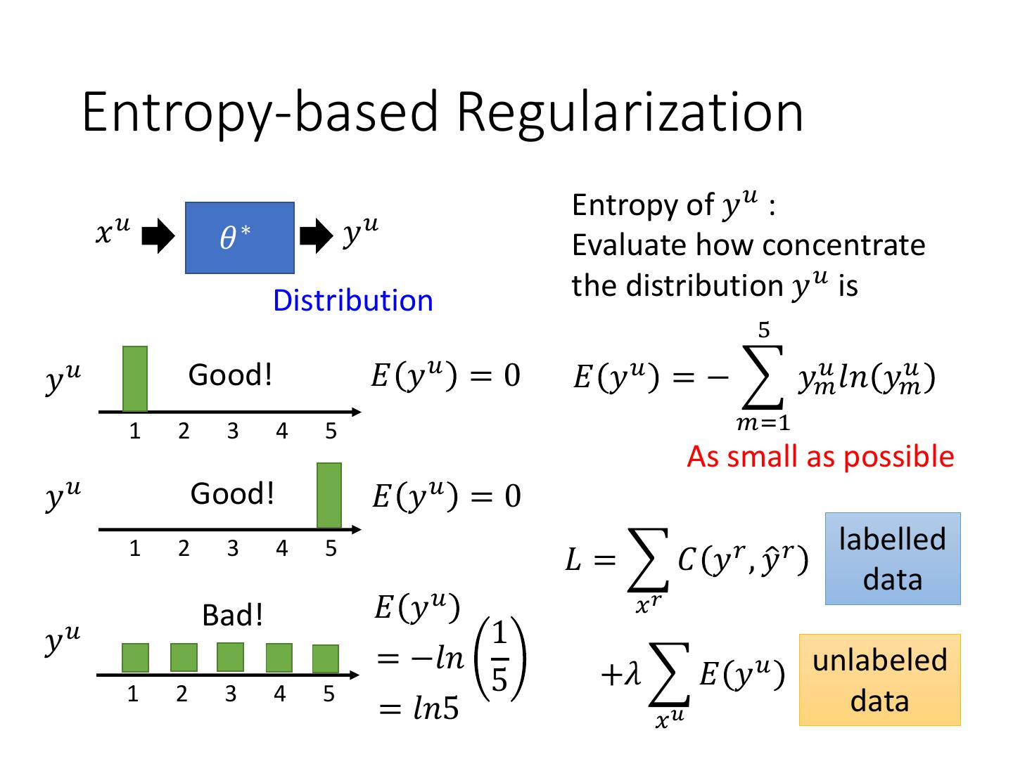
14 . Entropy-based Regularization Entropy of 𝑦 𝑢 : 𝑥𝑢 𝜃∗ 𝑦𝑢 Evaluate how concentrate Distribution the distribution 𝑦 𝑢 is 5 𝑦𝑢 Good! 𝐸 𝑦𝑢 = 0 𝐸 𝑦 𝑢 = − ෍ 𝑦𝑚 𝑢 𝑙𝑛 𝑦 𝑢 𝑚 1 2 3 4 5 𝑚=1 As small as possible 𝑦𝑢 Good! 𝐸 𝑦𝑢 = 0 labelled 1 2 3 4 5 𝐿 = ෍𝐶 𝑦 𝑟 , 𝑦ො 𝑟 data Bad! 𝐸 𝑦𝑢 𝑥𝑟 𝑦𝑢 1 = −𝑙𝑛 +𝜆 ෍ 𝐸 𝑦 𝑢 unlabeled 1 2 3 4 5 5 = 𝑙𝑛5 𝑥𝑢 data 

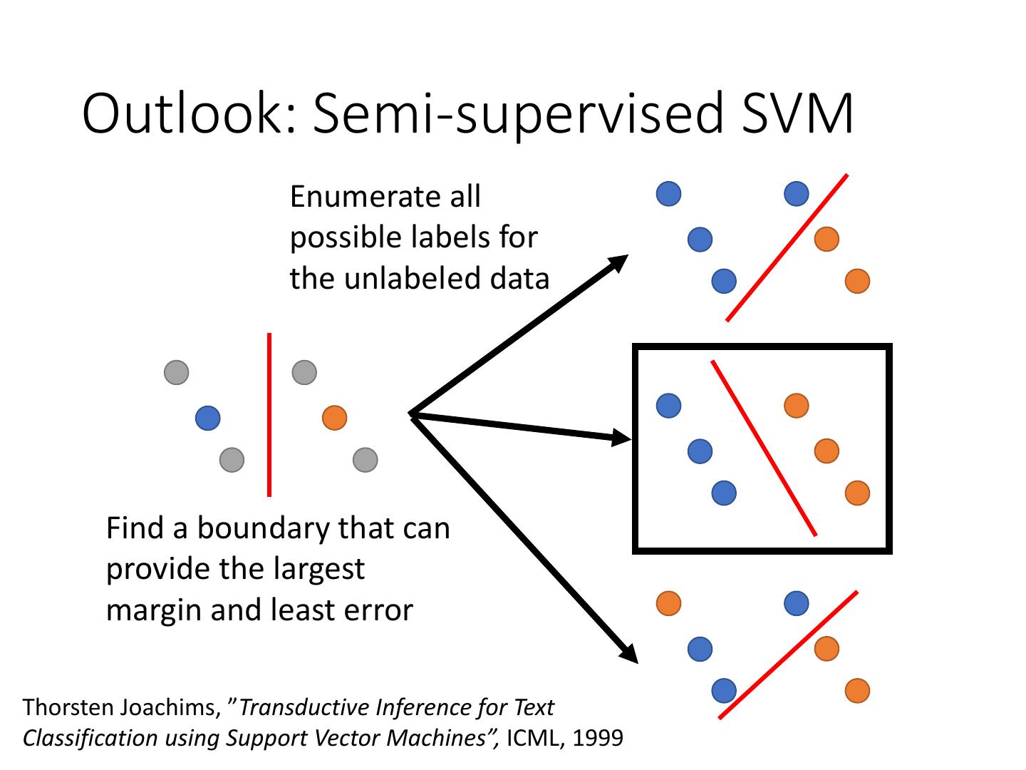
15 . Outlook: Semi-supervised SVM Enumerate all possible labels for the unlabeled data Find a boundary that can provide the largest margin and least error Thorsten Joachims, ”Transductive Inference for Text Classification using Support Vector Machines”, ICML, 1999 

16 .Semi-supervised Learning Smoothness Assumption 近朱者赤，近墨者黑 “You are known by the company you keep” 

17 . Smoothness Assumption • Assumption: “similar” 𝑥 has the same 𝑦ො • More precisely: • x is not uniform. • If 𝑥 1 and 𝑥 2 are close in a high density region, 𝑦ො 1 and 𝑦ො 2 are the same. connected by a high density path 公館 v.s. 台北車站 Source of image: 公館 v.s. 科技大樓 http://hips.seas.harvard.edu/files /pinwheel.png 

18 . Smoothness Assumption • Assumption: “similar” 𝑥 has the same 𝑦ො • More precisely: • x is not uniform. 𝑥3 • If 𝑥 1 and 𝑥 2 are close in 𝑥1 a high density region, 𝑦ො 1 and 𝑦ො 2 are the same. 𝑥2 connected by a high density path Source of image: 𝑥 1 and 𝑥 2 have the same label http://hips.seas.harvard.edu/files /pinwheel.png 𝑥 2 and 𝑥 3 have different labels 

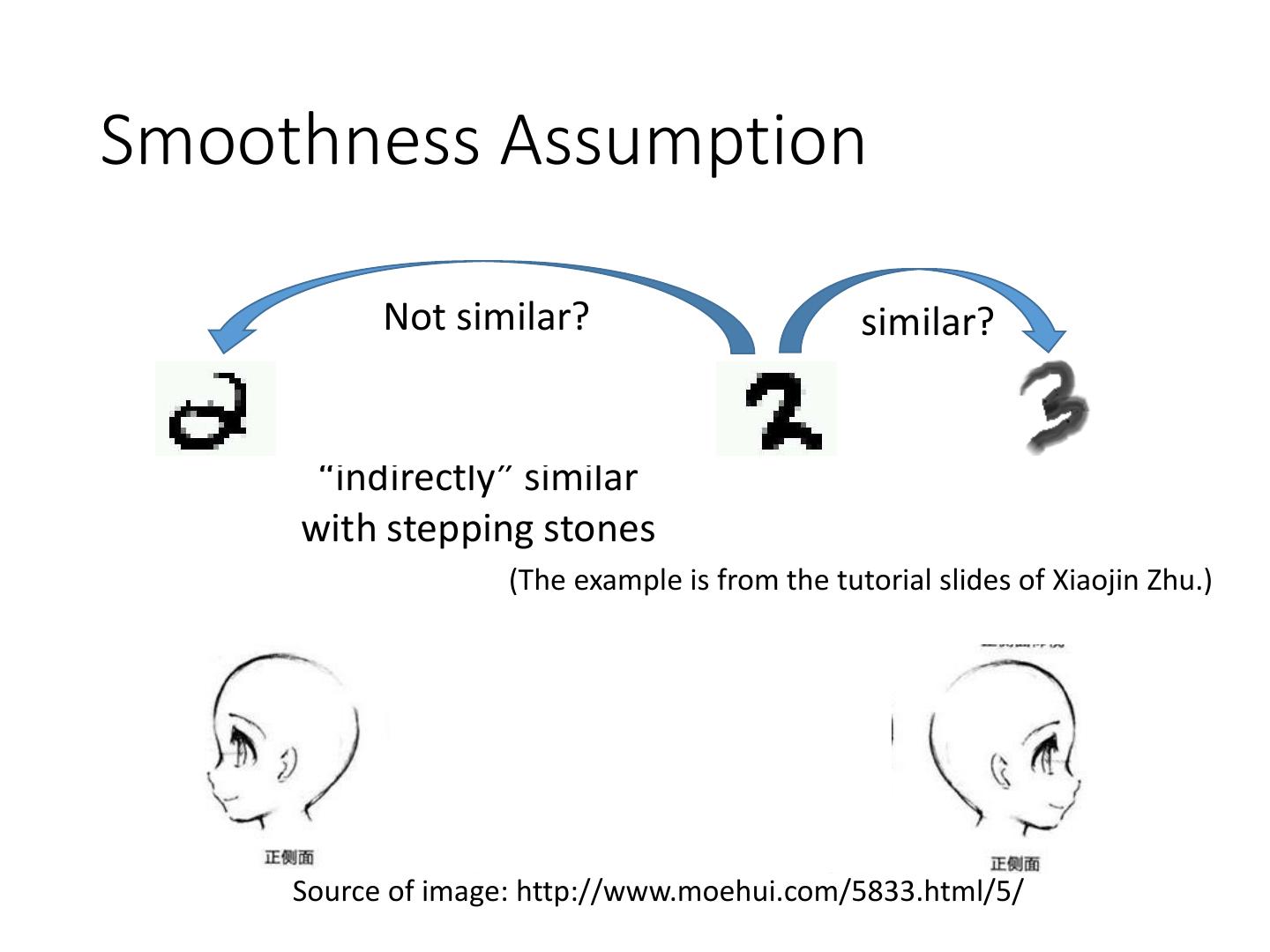
19 .Smoothness Assumption Not similar? similar? “indirectly” similar with stepping stones (The example is from the tutorial slides of Xiaojin Zhu.) Source of image: http://www.moehui.com/5833.html/5/ 

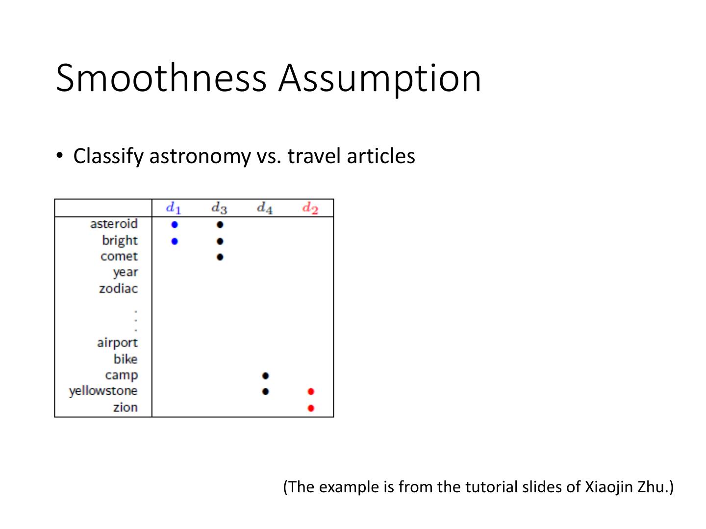
20 .Smoothness Assumption • Classify astronomy vs. travel articles (The example is from the tutorial slides of Xiaojin Zhu.) 

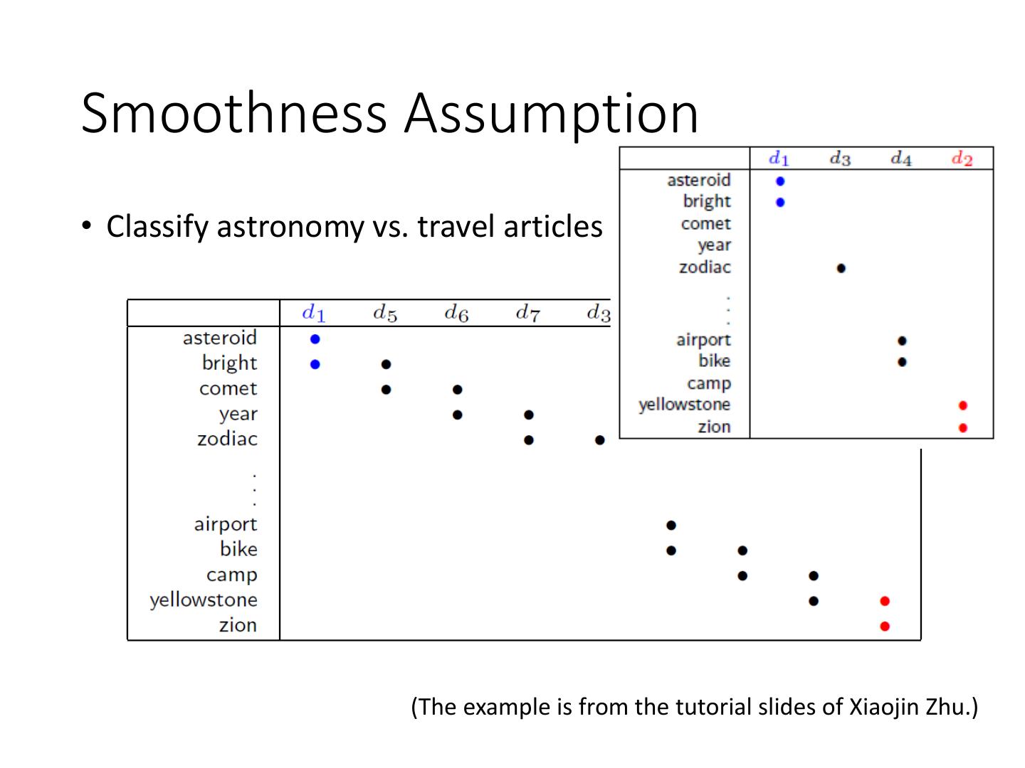
21 .Smoothness Assumption • Classify astronomy vs. travel articles (The example is from the tutorial slides of Xiaojin Zhu.) 

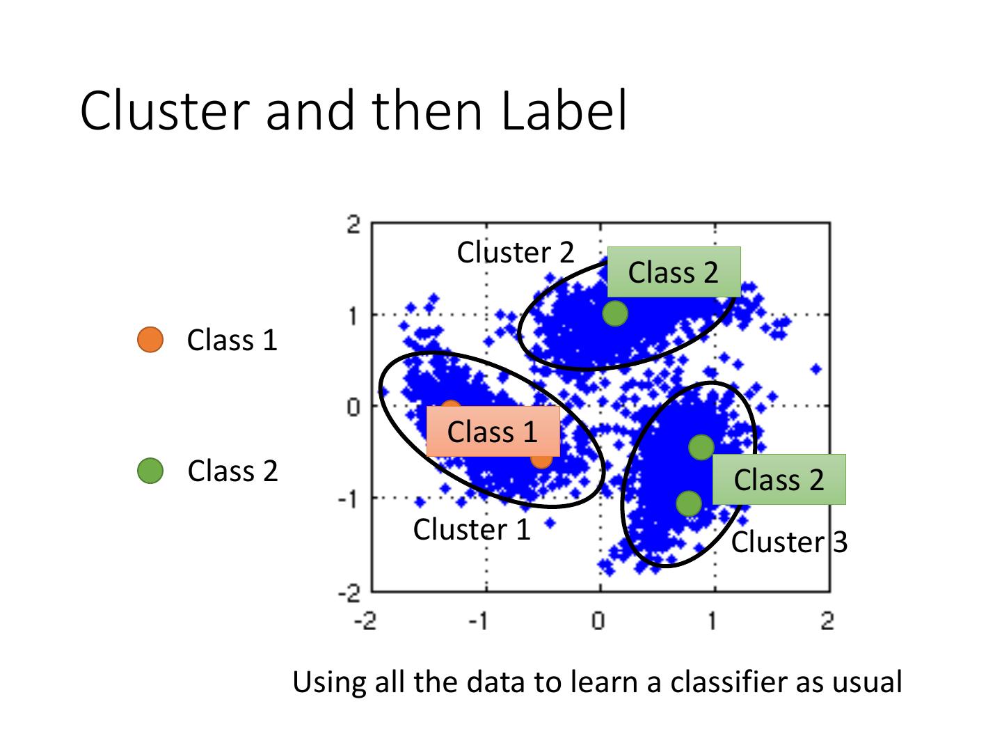
22 .Cluster and then Label Cluster 2 Class 2 Class 1 Class 1 Class 2 Class 2 Cluster 1 Cluster 3 Using all the data to learn a classifier as usual 

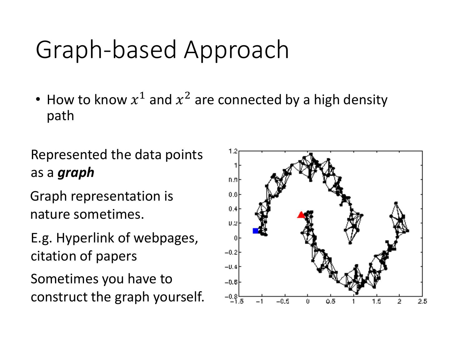
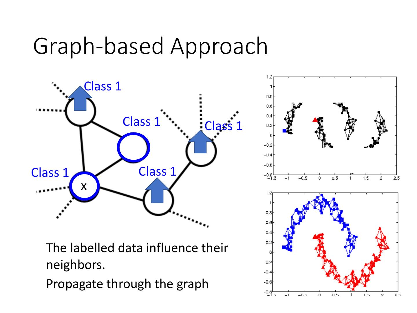
23 .Graph-based Approach • How to know 𝑥 1 and 𝑥 2 are connected by a high density path Represented the data points as a graph Graph representation is nature sometimes. E.g. Hyperlink of webpages, citation of papers Sometimes you have to construct the graph yourself. 

24 . The images are from the Graph-based Approach tutorial slides of Amarnag Subramanya and Partha - Graph Construction Pratim Talukdar • Define the similarity 𝑠 𝑥 𝑖 , 𝑥 𝑗 between 𝑥 𝑖 and 𝑥 𝑗 • Add edge: • K Nearest Neighbor • e-Neighborhood • Edge weight is proportional to s 𝑥 𝑖 , 𝑥 𝑗 Gaussian Radial Basis Function: 𝑖 𝑗 𝑖 𝑗 2 𝑠 𝑥 ,𝑥 = 𝑒𝑥𝑝 −𝛾 𝑥 − 𝑥 

25 .Graph-based Approach Class 1 Class 1 Class 1 Class 1 Class 1 x The labelled data influence their neighbors. Propagate through the graph 

26 . Graph-based Approach • Define the smoothness of the labels on the graph 1 𝑖 𝑗 2 𝑆 = ෍ 𝑤𝑖,𝑗 𝑦 − 𝑦 Smaller means smoother 2 𝑖,𝑗 For all data (no matter labelled or not) 𝑦1 =1 𝑦 1 = 0 x1 x1 3 2 3 𝑦3 =1 2 𝑦3 = 1 1 x3 1 x3 𝑦2 =1 x 2 𝑦 2 = 1 x2 1 1 x4 x4 𝑆 = 0.5 𝑆=3 𝑦4 = 0 𝑦4 =0 

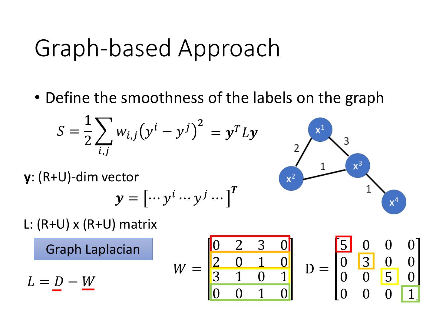
27 . Graph-based Approach • Define the smoothness of the labels on the graph 1 2 𝑆 = ෍ 𝑤𝑖,𝑗 𝑦 𝑖 − 𝑦 𝑗 = 𝒚𝑇 𝐿𝒚 2 𝑖,𝑗 y: (R+U)-dim vector 𝑻 𝒚 = ⋯ 𝑦𝑖 ⋯ 𝑦 𝑗 ⋯ L: (R+U) x (R+U) matrix Graph Laplacian 0 2 3 0 5 0 0 0 𝑊= 2 0 1 0 D= 0 3 0 0 𝐿 =𝐷−𝑊 3 1 0 1 0 0 5 0 0 0 1 0 0 0 0 1 

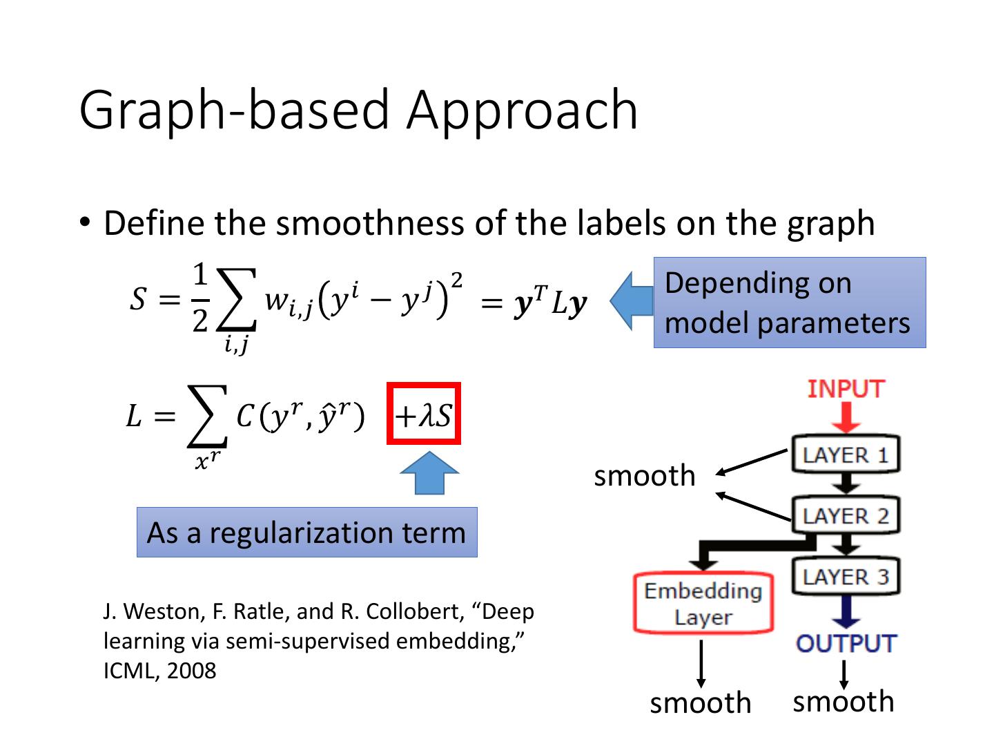
28 .Graph-based Approach • Define the smoothness of the labels on the graph 1 2 Depending on 𝑆 = ෍ 𝑤𝑖,𝑗 𝑦 𝑖 − 𝑦 𝑗 = 𝒚𝑇 𝐿𝒚 2 model parameters 𝑖,𝑗 𝐿 = ෍ 𝐶 𝑦 𝑟 , 𝑦ො 𝑟 +𝜆𝑆 𝑥𝑟 smooth As a regularization term J. Weston, F. Ratle, and R. Collobert, “Deep learning via semi-supervised embedding,” ICML, 2008 smooth smooth 

29 .Semi-supervised Learning Better Representation 去蕪存菁，化繁為簡