Explainable Recommendation Through Attentive Multi-View Learning

1 . Explainable Recommendation Through Attentive Multi-View Learning Jingyue Gao1,2 , Xiting Wang2 * , Yasha Wang1 , Xing Xie2 1 Peking University, {gaojingyue1997, wangyasha}@pku.edu.cn 2 Microsoft Research Asia, {xitwan, xing.xie}@microsoft.com Abstract Food Food High Fiber Food Meat Recommender systems have been playing an increasingly im- portant role in our daily life due to the explosive growth of in- Vegetable formation. Accuracy and explainability are two core aspects Seafood Dessert when we evaluate a recommendation model and have become Bread Fruit Green one of the fundamental trade-offs in machine learning. In this Oyster Steak Cake Pear Tomato paper, we propose to alleviate the trade-off between accuracy Shrimp Gelato Croissant Arugula and explainability by developing an explainable deep model that combines the advantages of deep learning-based models Figure 1: Multi-level user interest extracted using our method. The and existing explainable methods. The basic idea is to build hierarchies correspond to a 26-year-old female Yelp user (left) and an initial network based on an explainable deep hierarchy a 30-year-old male Yelp user (right). The features users care most (e.g., Microsoft Concept Graph) and improve the model accu- about are highlighted in orange. racy by optimizing key variables in the hierarchy (e.g., node importance and relevance). To ensure accurate rating predic- tion, we propose an attentive multi-view learning framework. The framework enables us to handle sparse and noisy data by and Yu 2017) achieve state-of-the-art accuracy due to co-regularizing among different feature levels and combining their capacity to model complex high-level features. How- predictions attentively. To mine readable explanations from ever, the high-dimensional high-level features they learn the hierarchy, we formulate personalized explanation genera- are beyond the comprehension of ordinary users. tion as a constrained tree node selection problem and propose • Explainable but shallow. Although many explainable a dynamic programming algorithm to solve it. Experimen- recommendation methods have been proposed, the ex- tal results show that our model outperforms state-of-the-art plainable components in the models are usually shallow. methods in terms of both accuracy and explainability. Typical explainable components include one or two layers of attention networks (Chen et al. 2017), matrix factoriza- Introduction tion (Zhang et al. 2014a), and topic modeling (McAuley and Leskovec 2013). They have achieved considerable Personalized recommendation has become one of the most success in improving explainability. However, the lack effective techniques to help users sift through massive of an effective mechanism to model high-level explicit amounts of web content and overcome information over- features limits their accuracy and/or explainability. These load. Recently, the recommendation community has reached methods can only select explanations from a pre-defined a consensus that accuracy can only be used to partially level of candidates. They cannot identify which level of evaluate a system. Explainability of the model, which is features best represents a user’s true interest. For example, the ability to provide explanations for why an item is rec- they are not able to tell whether a user only likes shrimps ommended, is considered equally important (Wang et al. (lower level) or is interested in seafood (higher level). 2018a). Appropriate explanations may persuade users to try In this paper, we aim to mitigate the trade-off between the item, increase users’ trust, and help users make better accuracy and explainability by developing an explainable decisions (Zhang et al. 2014a). deep model for recommendation. The model achieves state- Determining whether to optimize towards accuracy or ex- of-the-art accuracy and is highly explainable. Moreover, it plainability poses a fundamental dilemma for practitioners. enables us to accurately portray hierarchical user interest. As Currently, their choices are limited to two types of models: shown in Figure 1, the model can automatically infer multi- • Deep but unexplainable. Deep learning-based recom- level user profiles and identify which level of features best mendation models (Wang et al. 2017; Zheng, Noroozi, captures a user’s true interest, e.g., whether s/he is interested * Xiting Wang is the corresponding author in lower-level features such as shrimp or higher-level fea- Copyright © 2019, Association for the Advancement of Artificial tures such as seafood. Intelligence (www.aaai.org). All rights reserved. To design an explainable deep model as such, we are faced 

2 .with two major technical challenges. The first challenge is models (Kanagal et al. 2012; Zhang et al. 2014b). These to accurately model multi-level explicit features from noisy methods can effectively mitigate data sparsity. However, and sparse data. It is very difficult to model the relation- their accuracy and explainability are limited due to the lack ships between high-level and low-level features since they of a mechanism to model multi-level item features. have overlapping semantic meanings. For example, learning Recently, researchers have discovered that providing ex- whether seafood is important to the user is challenging be- planations may improve persuasiveness, effectiveness, ef- cause the user may only mention shrimp or meat in the re- ficiency and user trust (Zhang et al. 2014a). Thus, many view. The second challenge is to generate explanations that methods have been developed to improve the explainabil- are easy for common users to understand from the multi- ity of recommendation models (Ren et al. 2017; Peake and level structure. Wang 2018; Wang et al. 2018b). Pioneer works (McAuley To address these challenges, we develop a Deep Explicit and Leskovec 2013; Zhang et al. 2014a) focus on im- Attentive Multi-View Learning Model (DEAML). The basic proving the explainability of collaborative filtering models. idea is to build an initial network based on an explainable These works usually rely on shallow explainable compo- deep structure (e.g., knowledge graph) and improve accu- nents such as matrix factorization (Zhang et al. 2014a) and racy by optimizing key variables in the explainable structure generative models (Diao et al. 2014; Wu and Ester 2015) (e.g., node importance and relevance). To improve model for explanation generation. More recently, researchers dis- accuracy, we propose an attentive multi-view learning covered the attention mechanism’s capability in improving framework for rating prediction. In this framework, differ- the explainability of deep learning-based methods. By us- ent levels of features are considered as different views. Adja- ing the attention mechanism, the models can automatically cent views are connected by using the attention mechanism. learn the importance of explicit features and at the same Results from different views are co-regularized and atten- time refine user and/or item embeddings (Chen et al. 2017; tively combined to make the final prediction. This frame- 2018). Researchers have also built explainable models based work helps improve accuracy since it is robust to noise and on interpretable structures such as graphs (He et al. 2015) enables us to fully leverage the hierarchical information in and trees (Wang et al. 2018a). the explainable structure. Second, we formulate personal- The aforementioned explainable recommendation meth- ized explanation generation as a constrained tree node ods have achieved considerable success in improving ex- selection problem. To solve this problem, we propose a dy- plainability. However, to the best of our knowledge, none namic programming algorithm, which finds the optimal fea- of the existing explainable recommendation methods can tures for explanation in a bottom-up manner. model multi-level explicit (explainable) features. As a re- We conduct two experiments and a user study to evalu- sult, the accuracy and/or explainability of these methods are ate our method. Numerical experiments show that DEAML limited. Compared with these methods, our DEAML is an outperforms state-of-art deep learning-based recommenda- explainable deep model that achieves state-of-the-art accu- tion models in terms of accuracy. An evaluation with 20 hu- racy and meanwhile is highly explainable. Moreover, our man subjects has shown that the explanations generated by model can automatically learn multi-level user profile and us are considered significantly more useful than state-of-the- infer which level of features best captures a user’s interest. art aspect-based explainable recommendation method. Problem Definition Related Work We aim to build an explainable deep recommendation model Many methods have been proposed to improve recom- by incorporating an explicit (explainable) feature hierarchy. mendation accuracy, including content-based (Kompan and Input: The input of our model includes a user set U , an Bielikov´a 2010), collaborative filtering-based (Das et al. item set V , and an explicit feature hierarchy Υ. 2007) and hybrid methods (De Francisci Morales, Gionis, and Lucchese 2012). As an integration and extension of pre- Definition 1. An explicit feature hierarchy Υ is a tree vious methods, deep learning-based models are proposed where each node Fl is an explicit feature or aspect (e.g., to further improve accuracy. For example, CDL (Wang, meat) of the items (e.g., restaurants). Each edge is a tuple Wang, and Yeung 2015) jointly performs deep represen- (Fl1 , Fl2 ), which represents that the child Fl1 (e.g., beef) is tation leaning and collaborative filtering by employing a a sub-concept of the parent Fl2 (e.g., meat). We denote the hierarchical Bayesian model. He et al. propose a Neural set of nodes in Υ as F, where F = {F1 , ..., FL } and L rep- Collaborative Filtering framework to learn nonlinear in- resents the total number of nodes in Υ. teractions between users and items (He et al. 2017). In To build Υ, we leverage the Microsoft Concept DeepCoNN and NARRE (Zheng, Noroozi, and Yu 2017; Graph1 (Wu et al. 2012; Wang et al. 2015), which is a widely Chen et al. 2018), convolutional neural networks are lever- used knowledge graph with over 5 million concepts and 85 aged to extract features from textual reviews. Although these million “IsA” relations (e.g., cat IsA animal). We first map methods achieve significant improvement in accuracy, the n-grams in the reviews to concepts (or instances) in the con- high-level features extracted are beyond the understanding cept graph. Only the frequently used concepts that are highly of common users. Except for unstructured textual data, re- correlated with the ratings are kept and regarded as the ex- searchers have also designed models that leverage structural plicit features. We then recursively search the explicit fea- information. Famous examples are taxonomy-based meth- 1 ods that incorporate taxonomies of items into latent factor https://concept.research.microsoft.com/ 

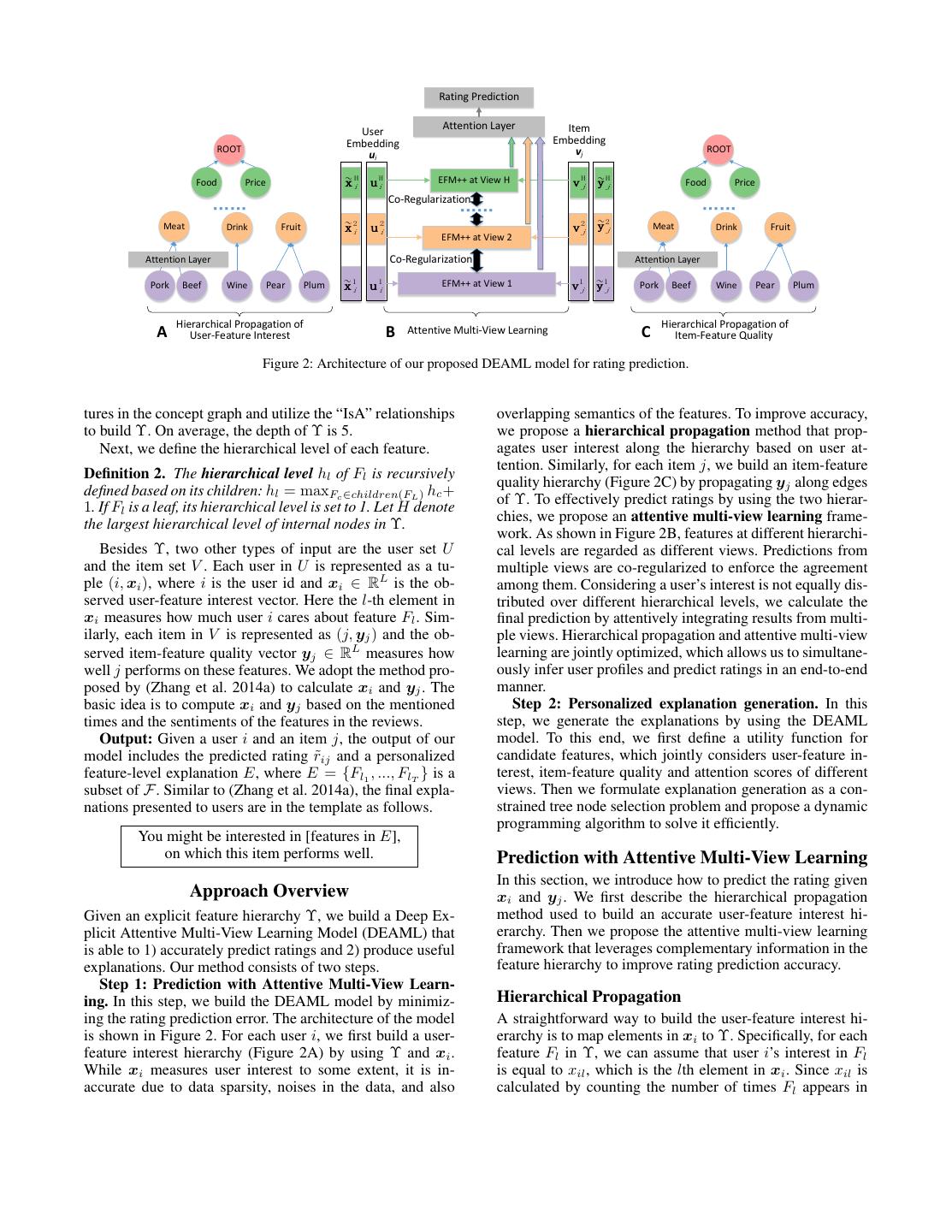
3 . Rating Prediction Attention Layer Item User Embedding Embedding ROOT vj ROOT ui H H Food Price ~i ui x EFM++ at View H v jH y ~j H Food Price Co-Regularization 2 Meat Drink Fruit x ~i 2 u i2 v j2 y ~j Meat Drink Fruit EFM++ at View 2 Attention Layer Co-Regularization Attention Layer 1 1 EFM++ at View 1 1 1 Pork Beef Wine Pear Plum x ~i ui vj y ~j Pork Beef Wine Pear Plum Hierarchical Propagation of Hierarchical Propagation of A User-Feature Interest B Attentive Multi-View Learning C Item-Feature Quality Figure 2: Architecture of our proposed DEAML model for rating prediction. tures in the concept graph and utilize the “IsA” relationships overlapping semantics of the features. To improve accuracy, to build Υ. On average, the depth of Υ is 5. we propose a hierarchical propagation method that prop- Next, we define the hierarchical level of each feature. agates user interest along the hierarchy based on user at- tention. Similarly, for each item j, we build an item-feature Definition 2. The hierarchical level hl of Fl is recursively quality hierarchy (Figure 2C) by propagating yj along edges defined based on its children: hl = maxFc ∈children(FL ) hc + of Υ. To effectively predict ratings by using the two hierar- 1. If Fl is a leaf, its hierarchical level is set to 1. Let H denote chies, we propose an attentive multi-view learning frame- the largest hierarchical level of internal nodes in Υ. work. As shown in Figure 2B, features at different hierarchi- Besides Υ, two other types of input are the user set U cal levels are regarded as different views. Predictions from and the item set V . Each user in U is represented as a tu- multiple views are co-regularized to enforce the agreement ple (i, xi ), where i is the user id and xi ∈ RL is the ob- among them. Considering a user’s interest is not equally dis- served user-feature interest vector. Here the l-th element in tributed over different hierarchical levels, we calculate the xi measures how much user i cares about feature Fl . Sim- final prediction by attentively integrating results from multi- ilarly, each item in V is represented as (j, yj ) and the ob- ple views. Hierarchical propagation and attentive multi-view served item-feature quality vector yj ∈ RL measures how learning are jointly optimized, which allows us to simultane- well j performs on these features. We adopt the method pro- ously infer user profiles and predict ratings in an end-to-end posed by (Zhang et al. 2014a) to calculate xi and yj . The manner. basic idea is to compute xi and yj based on the mentioned Step 2: Personalized explanation generation. In this times and the sentiments of the features in the reviews. step, we generate the explanations by using the DEAML Output: Given a user i and an item j, the output of our model. To this end, we first define a utility function for model includes the predicted rating r˜ij and a personalized candidate features, which jointly considers user-feature in- feature-level explanation E, where E = {Fl1 , ..., FlT } is a terest, item-feature quality and attention scores of different subset of F. Similar to (Zhang et al. 2014a), the final expla- views. Then we formulate explanation generation as a con- nations presented to users are in the template as follows. strained tree node selection problem and propose a dynamic programming algorithm to solve it efficiently. You might be interested in [features in E], on which this item performs well. Prediction with Attentive Multi-View Learning In this section, we introduce how to predict the rating given Approach Overview xi and yj . We first describe the hierarchical propagation Given an explicit feature hierarchy Υ, we build a Deep Ex- method used to build an accurate user-feature interest hi- plicit Attentive Multi-View Learning Model (DEAML) that erarchy. Then we propose the attentive multi-view learning is able to 1) accurately predict ratings and 2) produce useful framework that leverages complementary information in the explanations. Our method consists of two steps. feature hierarchy to improve rating prediction accuracy. Step 1: Prediction with Attentive Multi-View Learn- ing. In this step, we build the DEAML model by minimiz- Hierarchical Propagation ing the rating prediction error. The architecture of the model A straightforward way to build the user-feature interest hi- is shown in Figure 2. For each user i, we first build a user- erarchy is to map elements in xi to Υ. Specifically, for each feature interest hierarchy (Figure 2A) by using Υ and xi . feature Fl in Υ, we can assume that user i’s interest in Fl While xi measures user interest to some extent, it is in- is equal to xil , which is the lth element in xi . Since xil is accurate due to data sparsity, noises in the data, and also calculated by counting the number of times Fl appears in 

4 . x~il At level h, we employ an extended version of User EFM (Zhang et al. 2014a) to predict the rating based on Embedding ui Attention Layer ˜ hi and y˜jh . Compared with collaborative filtering, EFM en- x riches the user and item representations by adding an addi- tional set of latent factors learned from the explicit features. Feature Embedding e1 x~i 1 ec x~ic el x il Specifically, the user embedding for view h consists of two parts: uhi = phi ⊕ chi ∈ Rk . Here phi ∈ Rk1 are latent factors Children Parent learned from explicit features (explicit factors), chi ∈ Rk2 Figure 3: Hierarchical propagation of user interest. are implicit factors, and ⊕ is the concatenation operator. Similarly, the item embedding at level h is vjh = qjh ⊕ dhj , where qjh ∈ Rk1 denote the explicit factors and dhj ∈ Rk2 the reviews written by user i, this method captures user in- are the implicit factors. The explicit factors phi and qjh are terest to some extent. However, due to data sparsity, noises used to fit x ˜ hi with Z h phi and fit y˜jh with Z h qjh , where in the data, and overlapping semantics of features in Υ, the Z ∈Rh Lh ×k1 is the projection matrix of features at level h. constructed user-feature interest hierarchy can be inaccurate. Traditional EFM directly predicts the rating of user i on For instance, a user interested in meat may comment fre- quently on beef and pork but rarely mentions the word meat. item j as uhi vjh . We further extend it by incorporating To solve this issue, we infer users’ true interest x ˜ i by global average rating bias µ, user bias oi and item bias oj : propagating xi along Υ. For each parent Fl , we calculate h x ˜il by considering personalized user attention (Figure 3): r˜ij = uhi vjh + oi + oj + µ. (2) x ˜il = αll xil + αlc x ˜ic , Let Ω denote the set of training instances and rij denote the Fc ∈children(Fl ) ground-truth rating of user i on item j, the loss in view h is: exp(α∗ lc ) αlc = exp(α∗ ), (1) h F c ∈children(Fl )∪{Fl } lc Lh = λa i,j∈Ω (˜ rij − rij )2 + ∗ αlc = h1 ReLU (Wl el + Wc ec + Wu ui + b1 ) + b2 , λx ˜ hi − x Z h phi 2 + λy y˜jh − Z h qjh 2 , (3) i j where αlc is the attention score of feature Fc . el , ec ∈ Rd1 where λa , λx and λy are weights of corresponding items. are pre-trained embeddings of Fl and Fc . We follow the Co-regularization loss. We then consider how the mod- method proposed in (Choi et al. 2017) to train feature em- els in multiple views can complement each other. Based on beddings that capture both semantic and hierarchical infor- the consensus principle which aims to maximize the agree- mation. As there are H levels of features except FL in Υ, ment on multiple views (Xu, Tao, and Xu 2013), a common the user embedding at level h is uhi ∈ Rk and the global paradigm of multi-viewing learning is co-regularization. Ac- user embedding ui ∈ RkH is the concatenation of uhi at all tually, information distributed in different views describes levels (shown in Figure 2). The hidden layer size of the at- the inherent characteristics of user-feature interest and item- tention network is d2 . Wl ∈ Rd2 ×d1 , Wc ∈ Rd2 ×d1 , Wu ∈ feature quality from various aspects. We can regularize the Rd2 ×kH , h1 ∈ Rd2 , b1 ∈ Rd2 , b2 ∈ R and ui ∈ RkH are learning of multiple views by enforcing agreement among model parameters to be learned. their predictions. This way, complementary information can Propagation of yj is similar to that of xi . After that we be leveraged to benefit the learning of each single view. By obtain a more accurate item-feature quality vector y˜j . enforcing the agreement between two adjacent views, the co-regularization loss is: Attentive Multi-View Learning H−1 After we obtain accurate estimates of user-feature interest Lv = (˜h rij h+1 2 − r˜ij ) . (4) and item-feature quality, we predicate how much user i likes i,j∈Ω h=1 item j based on x ˜ i and y˜j . To accurately predict the rat- ing, we design an attentive multi-view learning framework. Joint learning. Predictions from multiple views should be In this section, we first introduce how to predict the ratings combined for the final prediction. One method is to aver- based on the information in a single view. Then, we describe age the predictions of all views. However, this assumes that the co-regularization loss that enforces agreement among each view contributes equally to the rating. In reality, differ- different views. Finally, we illustrate how to combine dif- ent views reveal user-feature interest and item-feature qual- ferent views in a unified model and learn parameters from ity at different levels of abstractness. The levels of interest different views jointly. also vary among users and items. Some users may care more Loss in each view. In our framework, each view consists about general features (e.g. food and service) while others of features at the same hierarchical level. We first consider may be more attracted by a specific feature (e.g. beef ). This rating prediction in a single view. Suppose there are Lh is the same for items. The views are not equally useful and features at level h. By only considering users’ interest on should be assigned different weights. The weights are sup- these features, we obtain a local user-feature interest vector posed to be determined in a user-item-specific way to bet- x˜ hi ∈ RLh , which is a slice of x˜ i . Similarly, we can obtain ter consider users’ interest and items’ quality. Thus we use y˜jh ∈ RLh , which is a slice of y˜j . the attention mechanism to combine multiple views. Let Ih 

5 .denote the H-dimensional one-hot vector for view h. The the total utility score of the selected features. We further re- attention network for view combination is: quire that features (e.g. beef ) cannot be selected simultane- ously with their ancestors in Υ (e.g. meat) since they are se- wh∗ = h2 ReLU (W1 ui + W2 vj + W3 Ih + b3 ) + b4 , mantically overlapping. Mathematically, we formulate per- ∗ exp(wh ) sonalized explanation generation as a constrained tree node wh = H exp(wh∗ ). (5) h =1 selection problem: L where ui , vj ∈ RkH are the global user embedding and argmax l=1 (φl Ψ(Fl )) , item embedding used in hierarchical propagation. W1 ∈ φ1 ,...,φL Rd3 ×kH , W2 ∈ Rd3 ×kH , W3 ∈ Rd3 ×H , h2 ∈ Rd3 , b3 ∈ L s.t. l=1 φl = T, φl ∈ {0, 1}, (9) Rd3 , b4 ∈ R are model parameters and d3 is the hidden φl1 φl2 Anc(l1 , l2 ) = 0, ∀ hl1 < hl2 , layer size of this attention network. The final prediction is a weighted sum of predictions in each view, where wh is the where φl = 1 (φl = 0) means feature Fl is (not) selected weight of view h: and Anc(l1 , l2 ) returns 1 if Fl2 is an ancestor of Fl1 . We solve the above problem by using dynamic program- H ming. Let G(l, t) denote the maximum utility we can obtain h r˜ij = wh r˜ij . (6) by selecting t nodes in the subtree rooted at Fl . Let us use h=1 IDls to represent the id of the s-th child feature of Fl , em- ploy J(l, s, t) to denote the maximum utility we can obtain Let Θ 2 denote the L2 norm of all parameters in our by selecting t nodes from the first s children of Fl , and use model. We optimize the following objective function: S to denote the total number of children of Fl . We have the H following transition equations: L= rij − rij )2 + (˜ Lh + λv Lv + λr Θ 2 , (7) max (Ψ(Fl ), J(l, S, t)) t = 1 i,j∈Ω h=1 G(l, t) = (10) J(l, S, t) t>1 where λv , λr are weights of corresponding items. We use the J(l, s, t) = max (J(l, s − 1, t ) + G(IDls , t − t )) . Adam optimizer (Kingma and Ba 2014) because it can auto- 0 t t matically adjust the learning rate during the training phase. Here, we need to carefully consider whether t = 1 because if we select more than one node (i.e., t >1) from the sub- Personalized Explanation Generation tree rooted at Fl , Fl itself can not be selected. Otherwise, The goal of personalized explanation generation is to select the constraint will be violated. Supposing that the root of Υ T features from Υ that are most useful in helping user i is FL , we can obtain the final solution with the maximum decide whether s/he will try item j. Selecting features dis- utility G(L,T) by using Equation (10) iteratively. tributed in multiple hierarchical levels is challenging be- Time complexity. If the maximum number of children of a cause 1) users’ interest is not evenly distributed over differ- feature is M , the time complexity of our dynamic program- ent hierarchical levels and 2) we need to avoid selecting fea- ming algorithm is O(LM T 2 ). It is more efficient than the tures with overlapping semantics. In this section, we first in- brute force algorithm whose time complexity is O(LT ). troduce our utility function, which estimates the usefulness of each feature. Then, we formulate the feature selection as Experiments a constrained tree node selection problem and propose a dy- We conduct two experiments and a user study to evaluate the namic programming method to solve it efficiently. effectiveness of our method. First, we demonstrate that our Utility function. Given user i and item j, three factors are method performs better than the state-of-the-art methods in considered when judging whether a feature Fl is useful: terms of accuracy. Then, we conduct parameter sensitivity • Whether user i is interested in Fl . analysis to validate the robustness of our model. Finally, we • How well item j performs on Fl . evaluate the explainability of DEAML with 20 human sub- • The weight of the view that Fl belongs to. jects in a user study. In view h, the explicit factors phi and qjh are used to fit the Table 1: Statistics of three public datasets. user-interest vector x˜ hi with Z h phi and fit y˜jh with Z h qjh . Let Fl be the ˆl-th feature at level h. We define the utility Dataset #Users #Items #Reviews score of Fl in the recommendation instance (i, j) as: Toys and Games 19,412 11,924 167,597 Digital Music 5,541 3,568 64,706 Ψ(Fl ) = Z h phi ˆl Z h qjh ˆl wh , (8) Yelp 8,744 14,082 212,922 where wh is the user-item-specific attention weight for view h, which is calculated by using Equation (5). The utility Experimental Settings score for the root feature is set to 0 since it does not have a Datasets. We use three datasets from different domains for concrete meaning. This utility function jointly incorporates evaluation. Table 1 summarizes the statistics of the datasets. three factors mentioned above. • Toys and Games is the part of the Amazon dataset2 that Constrained tree node selection. Next, we select T features 2 to be included in the explanation. The goal is to maximize http://jmcauley.ucsd.edu/data/amazon 

6 . Table 2: RMSE comparison with baselines on three datasets. Best results are highlighted in bold. G1 G2 G3 Ours NMF PMF SVD++ CKE HFT EFM DeepCoNN NARRE DEAML-V DEAML . Toys and Games 1.1489 1.1832 0.9071 0.9923 0.9958 0.9534 0.9199 0.9084 0.9062 0.9040 Digital Music 1.1520 1.2619 0.9211 0.9849 1.0910 0.9696 0.9212 0.9209 0.9190 0.9118 Yelp 1.2678 1.2413 1.1561 1.2279 1.2738 1.2019 1.1503 1.1348 1.1343 1.1333 focuses on Toys and Games. We choose the 5-core version ratings and keep only top-500 of them. We set d1 , d2 , d3 , λv , where all users and items have at least 5 reviews. and λa to 20, 10, 10, 10.0, and 3.0, respectively. • Digital Music is also from the Amazon 5-core dataset. It focuses on the domain of digital music. Study on Model Accuracy • Yelp consists of restaurant reviews from Yelp Challenge Overall performance. The accuracy of our approach and 20183 . Since the raw data is very large and sparse, we the baselines on three datasets are shown in Table 2. After follow (Zhang et al. 2014a) to preprocess the data. Specif- analyzing the results, we made the following conclusions. ically, we select restaurants located in the Phoenix city First, methods that incorporate review information (G3) and ensure that all users and items have at least 10 ratings. generally perform better than others. Compared with those Baselines. We select eight competitive methods for compar- only relying on a rating matrix (G1) and the method that ison. These methods can be divided into three groups ac- incorporates the feature hierarchy (G2), methods in G3 re- cording to the type of data they use. spectively achieve 8.9% and 3.0% improvement in accuracy • The first group (G1) only relies on the observed rating on average. We ascribe this to the fact that reviews provide matrix for rating prediction. This group consists of three more information about users’ interest and items’ quality. methods: NMF (Lee and Seung 2001), PMF (Mnih and Second, deep recommendation models (DeepCoNN, Salakhutdinov 2008) and SVD++ (Koren 2008). NARRE and ours) perform significantly better than those • The second group (G2) contains a knowledge-based with shallow models (10.7% improvement in accuracy on method, CKE (Zhang et al. 2016). Here, we regard the average). This is because deep models can model high-level feature hierarchy Υ as the structural knowledge in CKE. features more effectively and better capture non-linear inter- • The third group (G3) consists of four methods that actions. This again demonstrates the necessity of developing leverage the textual reviews for rating prediction: a deep version of the explainable models. HFT (McAuley and Leskovec 2013), EFM (Zhang et al. Third, our DEAML model achieves the best performance 2014a), DeepCoNN (Zheng, Noroozi, and Yu 2017) and on all three datasets. Our approach performs significantly NARRE (Chen et al. 2018). Among them, DeepCoNN better than EFM, achieving 5.7%, 5.2% and 6.0% improve- and NARRE are deep learning-based. EFM is the state-of- ments on three datasets. This demonstrates the effective- the-art method for mining feature-level explanations from ness of our attentive multi-view learning framework. While a single layer of features (no hierarchical structure). EFM predicts ratings from a single view, our design of at- Evaluation metric. We adopt the widely-used Root Mean tentive multi-view learning allows different views to com- Square Error (RMSE) to evaluate the accuracy of all algo- plement and benefit each other. Compared with CKE that rithms on rating prediction. A lower RMSE indicates a better simply learns item embeddings from knowledge bases, our performance. This is calculated as: approach fully leverages the feature hierarchy and improves 1 accuracy by 8.0%. The infusion of explicit feature hierarchy RM SE = rij − rij )2 , (˜ (11) provides our approach with additional knowledge that Deep- N i,j CoNN and NARRE cannot leverage. Given a set of explicit where N is the total number of testing instances. features, DEAML can differentiate low-level features from Details. We randomly split the dataset into training (70%), high-level ones and learn the associations between the fea- validation (15%) and test (15%) sets. We tune the hyper- tures, while DeepCoNN and NARRE treat all features as if parameters of each algorithm on the validation set and eval- they are at the same level. On average, our method is 1.0% uate their performance on the test set. The number of latent more accurate than DeepCoNN and NARRE. factors k for algorithms is searched in [8,16,32,64,128]. Af- Effectiveness of the attention mechanism. In DEAML, ter parameter tuning, we set k = 8 for NMF, PMF and HFT, we employ the attention mechanism to combine predictions and k = 16 for SVD++. We set k = 32 for EFM, CKE, from different views. To validate the effectiveness of the at- DeepCoNN, NARRE and DEAML. We reuse most hyper- tention mechanism, we design DEAML-V, which is a vari- parameters of DeepCoNN and NARRE reported by their au- ant that assigns same weights to all views. From Table 2 we thors. For simplicity, the number of explicit and implicit fac- can observe that DEAML constantly performs better than tors are set equally in EFM and DEAML. When constructing DEAML-V. It verifies our consideration that different views Υ in DEAML, we select the top-2000 frequently mentioned contain features at different levels of abstractness and should concepts in reviews, sort them by their correlations with the be assigned weights according to users’ interest and items’ quality. The attention mechanism enables DEAML to com- 3 https://www.yelp.com/dataset/challenge bine multiple views more adaptively and perform better. 

7 . DEAML ipants who have written at least 15 Yelp reviews. The par- 0.95 ticipants are independent and do not know each other. All SVD++ 0.94 DeepCoNN reviews on the restaurants they mentioned are crawled and NARRE RMSE merged with other reviews in the Yelp dataset. Two baselines 0.93 are used for comparison. The first baseline is PAV, which 0.92 is the famous “People Also Viewed” explanation. The sec- ond baseline is EFM, which is the state-of-the-art method for 0.91 8 16 32 64 128 generating feature-level explanations. We apply our method Number of latent factors and baselines on the merged dataset and randomly sample 100 restaurants for testing. We ensure that none of the partic- Figure 4: RMSE on Digital Music with different numbers of latent ipants go to these restaurants. For each restaurant, we gener- factors (compared with three competitive baselines). ate three explanations for each participant using PAV, EFM, and DEAML. The template of EFM is same as DEAML and PAV has it own format:“People also viewed this item”. T is 0.915 0.919 set to 3 for both EFM and DEAML. The participants are re- quired to give annotations from 1 to 5 on each explanation RMSE RMSE 0.913 0.915 according to its usefulness in helping them decide whether they will go to the restaurants. We randomly shuffle the order 0.911 0.911 of explanations so that they do not know which explanation comes from which method4 . 0 10 20 30 40 50 0 1 2 3 4 5 v a Table 3: Average score on explanation usefulness. <30 and ≥30 refer to two age groups. Figure 5: RMSE on Digital Music with different weights λv of co- regularization (left) and weights λa of errors in each view (right). Male Female <30 ≥30 Overall . PAV 1.35 1.51 1.65 1.11 1.41 EFM 3.18 3.13 3.03 3.32 3.16 Parameter Sensitivity Analysis DEAML 3.69 3.52 3.58 3.68 3.63 In this section, we study the sensitivity of several important parameters in our approach. We only report results on Digi- Table 3 shows the average score on the usefulness of tal Music here due to the space limitation. Results on other explanations generated by the three methods. We observe datasets are similar. that PAV performs the worst since it only suggests that one Effect of number of latent factors. We first compare our restaurant is popular and is not personalized. Our DEAML approach with three competitive baselines (SVD++, Deep- outperforms EFM in explanation usefulness (14.9% im- CoNN and NARRE) at different numbers of latent factors. provement). This suggests that DEAML can accurately iden- The results are shown in Figure 4. We can see that DEAML tify a user’s interest and a restaurant’s quality on multi-level consistently achieves the best performance with varying features while EFM suffers from the sparse and noisy data. numbers of latent factors. This demonstrates the robustness Additionally, EFM often selects features that are semanti- of our approach. We further observe that increasing the num- cally overlapped (e.g., food and cheese) since it ignores the ber of latent factors does not necessarily improve accuracy, hierarchical structure of features while DEAML considers because too many latent factors may lead to over fitting. such constraints to make the generated explanation more in- Effectiveness of co-regularization. We then study how formative. We also study the annotations given by partici- RMSE changes with λv , which is the weight of the co- pants of different profiles such as gender and age (see Table regularization loss term. The left part of Figure 5 shows 3). DEAML consistently performs the best for both male and that our approach achieves the best performance when λv female participants. It is the same for participants in the two is 10.0. Smaller or larger λv will hurt performance. This age groups. This suggests that DEAML is robust to various demonstrates the importance of involving agreement (co- user profiles and is personalized enough to generate useful regularization) among different views. explanations that help each user make better decisions. Effectiveness of enforcing accurate prediction in each view. The right part of Figure 5 shows how RMSE changes Conclusions with increasing λa , which is the weight of rating prediction errors in each single view. The lowest RMSE is achieved In this paper, we propose a Deep Explicit Attentive Multi- when λa = 3.0. When λa is 0, the performance degrades View Learning Model (DEAML) for explainable rec- since we fail to train a good predictor in each single view. ommendation, which combines the advantages of deep learning-based methods and existing explainable methods. Study on Explainability The proposed attentive multi-view learning frameworks en- ables the model to accurately predict ratings and infer multi- In this section, we evaluate the usefulness of our explana- tions in helping real-world users make better decisions.With 4 Explanations generated are at https://www.microsoft.com/en- the help of a data annotation company, we recruit 20 partic- us/research/uploads/prod/2018/10/explanations.csv 

8 .level user profiles. To support personalized explanation gen- McAuley, J., and Leskovec, J. 2013. Hidden factors and eration from multi-level features, we formulate the problem hidden topics: understanding rating dimensions with review as constrained tree node selection and solve it efficiently text. In RecSys, 165–172. ACM. by using dynamic programming. Experimental results show Mnih, A., and Salakhutdinov, R. R. 2008. Probabilistic ma- that our model performs better than state-of-the-art methods trix factorization. In NIPS, 1257–1264. in both accuracy and explainability. Peake, G., and Wang, J. 2018. Explanation mining: Post hoc interpretability of latent factor models for recommendation Acknowledgments systems. In SIGKDD, 2060–2069. ACM. This work is supported by the National Natural Science Ren, Z.; Liang, S.; Li, P.; Wang, S.; and de Rijke, M. 2017. Foundation of China (Grant No. 61772045). Social collaborative viewpoint regression with explainable recommendations. In WSDM, 485–494. ACM. References Wang, Z.; Wang, H.; Wen, J.-R.; and Xiao, Y. 2015. An in- Chen, J.; Zhang, H.; He, X.; Nie, L.; Liu, W.; and Chua, ference approach to basic level of categorization. In CIKM, T.-S. 2017. Attentive collaborative filtering: Multimedia 653–662. ACM. recommendation with item-and component-level attention. Wang, X.; Yu, L.; Ren, K.; Tao, G.; Zhang, W.; Yu, Y.; and In SIGIR, 335–344. ACM. Wang, J. 2017. Dynamic attention deep model for article recommendation by learning human editors’ demonstration. Chen, C.; Zhang, M.; Liu, Y.; and Ma, S. 2018. Neural In SIGKDD, 2051–2059. ACM. attentional rating regression with review-level explanations. In WWW, 1583–1592. International World Wide Web Con- Wang, X.; He, X.; Feng, F.; Nie, L.; and Chua, T.-S. 2018a. ferences Steering Committee. Tem: Tree-enhanced embedding model for explainable rec- ommendation. In WWW, 1543–1552. International World Choi, E.; Bahadori, M. T.; Song, L.; Stewart, W. F.; and Sun, Wide Web Conferences Steering Committee. J. 2017. Gram: graph-based attention model for healthcare representation learning. In SIGKDD, 787–795. ACM. Wang, X.; Chen, Y.; Yang, J.; Wu, L.; Wu, Z.; and Xie, X. 2018b. A reinforcement learning framework for explainable Das, A. S.; Datar, M.; Garg, A.; and Rajaram, S. 2007. recommendation. In ICDM. IEEE. Google news personalization: scalable online collaborative filtering. In WWW, 271–280. ACM. Wang, H.; Wang, N.; and Yeung, D.-Y. 2015. Collaborative deep learning for recommender systems. In SIGKDD, 1235– De Francisci Morales, G.; Gionis, A.; and Lucchese, C. 1244. ACM. 2012. From chatter to headlines: harnessing the real-time web for personalized news recommendation. In WSDM, Wu, Y., and Ester, M. 2015. Flame: A probabilistic model 153–162. ACM. combining aspect based opinion mining and collaborative filtering. In WSDM, 199–208. Diao, Q.; Qiu, M.; Wu, C.-Y.; Smola, A. J.; Jiang, J.; and Wu, W.; Li, H.; Wang, H.; and Zhu, K. Q. 2012. Probase: A Wang, C. 2014. Jointly modeling aspects, ratings and senti- probabilistic taxonomy for text understanding. In SIGMOD, ments for movie recommendation. In SIGKDD, 193–202. 481–492. ACM. He, X.; Chen, T.; Kan, M.-Y.; and Chen, X. 2015. Trirank: Xu, C.; Tao, D.; and Xu, C. 2013. A survey on multi-view Review-aware explainable recommendation by modeling as- learning. arXiv preprint arXiv:1304.5634. pects. In CIKM, 1661–1670. ACM. Zhang, Y.; Lai, G.; Zhang, M.; Zhang, Y.; Liu, Y.; and Ma, He, X.; Liao, L.; Zhang, H.; Nie, L.; Hu, X.; and Chua, T.- S. 2014a. Explicit factor models for explainable recommen- S. 2017. Neural collaborative filtering. In WWW, 173– dation based on phrase-level sentiment analysis. In SIGIR, 182. International World Wide Web Conferences Steering 83–92. ACM. Committee. Zhang, Y.; Ahmed, A.; Josifovski, V.; and Smola, A. 2014b. Kanagal, B.; Ahmed, A.; Pandey, S.; Josifovski, V.; Yuan, J.; Taxonomy discovery for personalized recommendation. In and Garcia-Pueyo, L. 2012. Supercharging recommender WSDM, 243–252. ACM. systems using taxonomies for learning user purchase behav- ior. Proceedings of the VLDB Endowment 5(10):956–967. Zhang, F.; Yuan, N. J.; Lian, D.; Xie, X.; and Ma, W.-Y. 2016. Collaborative knowledge base embedding for recom- Kingma, D. P., and Ba, J. 2014. Adam: A method for mender systems. In SIGKDD, 353–362. ACM. stochastic optimization. arXiv preprint arXiv:1412.6980. Zheng, L.; Noroozi, V.; and Yu, P. S. 2017. Joint deep mod- Kompan, M., and Bielikov´a, M. 2010. Content-based news eling of users and items using reviews for recommendation. recommendation. In International conference on electronic In WSDM, 425–434. ACM. commerce and web technologies, 61–72. Springer. Koren, Y. 2008. Factorization meets the neighborhood: a multifaceted collaborative filtering model. In SIGKDD, 426–434. ACM. Lee, D. D., and Seung, H. S. 2001. Algorithms for non- negative matrix factorization. In NIPS, 556–562.