Plug & Play Generative Networks

1 . Plug & Play Generative Networks: Conditional Iterative Generation of Images in Latent Space Anh Nguyen Jeff Clune Yoshua Bengio † † University of Wyoming Uber AI Labs , University of Wyoming Montreal Institute for Learning Algorithms anh.ng8@gmail.com jeffclune@uwyo.edu yoshua.umontreal@gmail.com Alexey Dosovitskiy Jason Yosinski arXiv:1612.00005v2 [cs.CV] 12 Apr 2017 University of Freiburg Uber AI Labs† dosovits@cs.uni-freiburg.de yosinski@uber.com Abstract Generating high-resolution, photo-realistic images has been a long-standing goal in machine learning. Recently, Nguyen et al. [37] showed one interesting way to synthesize novel images by performing gradient ascent in the latent space of a generator network to maximize the activations of one or multiple neurons in a separate classifier network. In this paper we extend this method by introducing an addi- tional prior on the latent code, improving both sample qual- ity and sample diversity, leading to a state-of-the-art gen- erative model that produces high quality images at higher resolutions (227 × 227) than previous generative models, and does so for all 1000 ImageNet categories. In addition, we provide a unified probabilistic interpretation of related activation maximization methods and call the general class of models “Plug and Play Generative Networks.” PPGNs are composed of 1) a generator network G that is capable Figure 1: Images synthetically generated by Plug and Play of drawing a wide range of image types and 2) a replace- Generative Networks at high-resolution (227x227) for four able “condition” network C that tells the generator what ImageNet classes. Not only are many images nearly photo- to draw. We demonstrate the generation of images condi- realistic, but samples within a class are diverse. tioned on a class (when C is an ImageNet or MIT Places classification network) and also conditioned on a caption 1. Introduction (when C is an image captioning network). Our method also improves the state of the art of Multifaceted Feature Visual- Recent years have seen generative models that are in- ization [40], which generates the set of synthetic inputs that creasingly capable of synthesizing diverse, realistic images activate a neuron in order to better understand how deep that capture both the fine-grained details and global coher- neural networks operate. Finally, we show that our model ence of natural images [54, 27, 9, 15, 43, 24]. However, performs reasonably well at the task of image inpainting. many important open challenges remain, including (1) pro- While image models are used in this paper, the approach is † This work was mostly performed at Geometric Intelligence, which modality-agnostic and can be applied to many types of data. Uber acquired to create Uber AI Labs. 1 

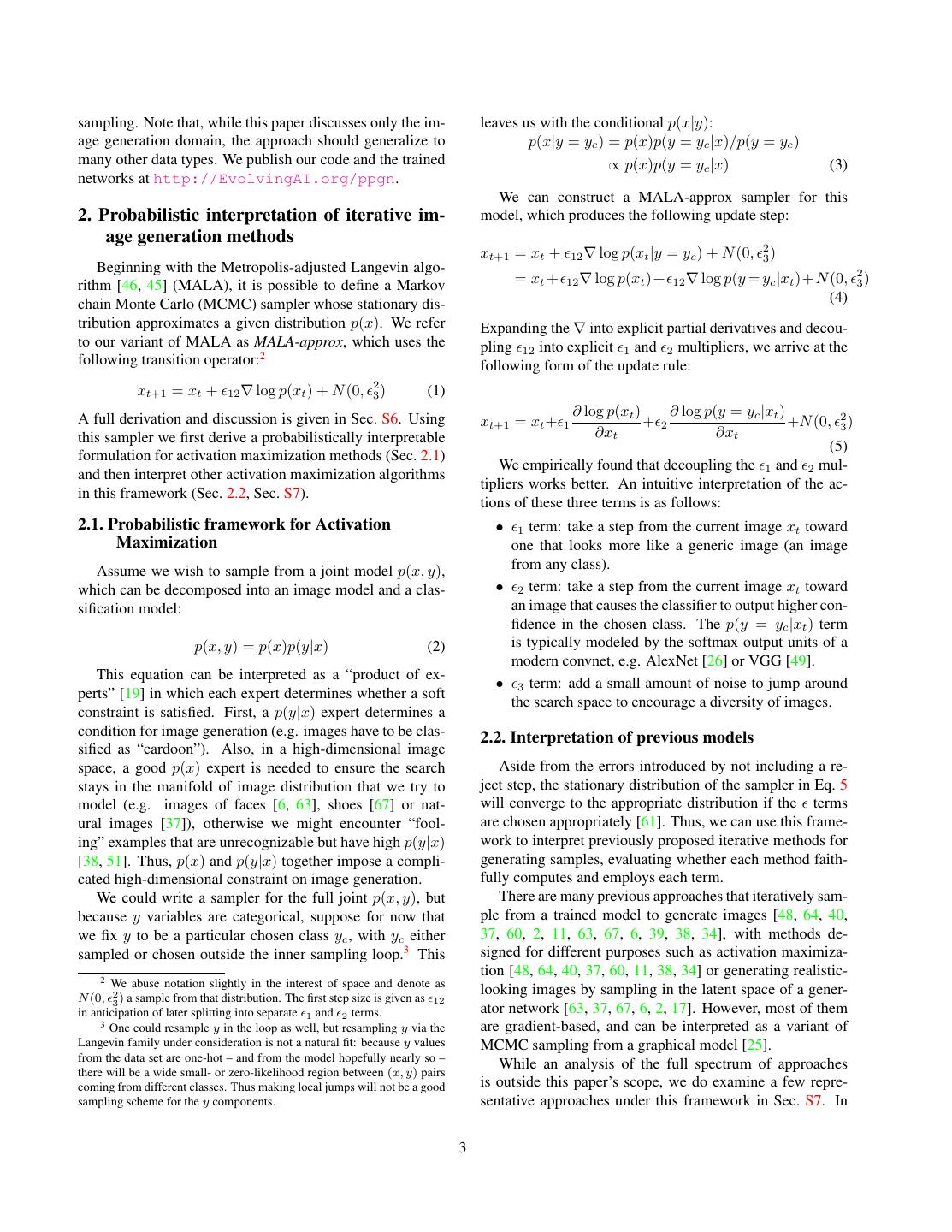
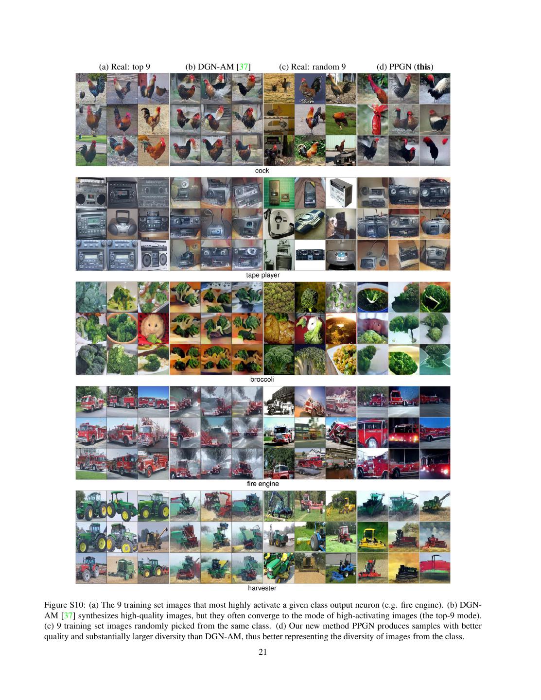
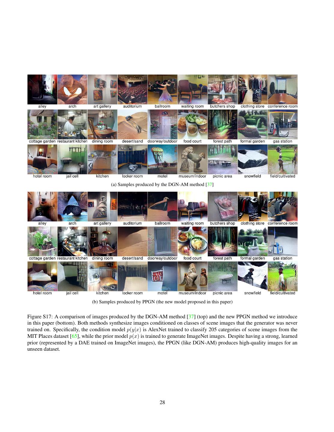
2 . (a) Real: top 9 (b) DGN-AM [37] (c) Real: random 9 (d) PPGN (this) Figure 2: For the “cardoon” class neuron in a pre-trained ImageNet classifier, we show: a) the 9 real training set images that most highly activate that neuron; b) images synthesized by DGN-AM [37], which are of similar type and diversity to the real top-9 images; c) random real training set images in the cardoon class; and d) images synthesized by PPGN, which better represent the diversity of random images from the class. Fig. S10 shows the same four groups for other classes. ducing photo-realistic images at high resolutions [30], (2) closeup of a single cardoon plant with a green background). training generators that can produce a wide variety of im- It is noteworthy that the images produced by DGN-AM ages (e.g. all 1000 ImageNet classes) instead of only one or closely match the images from that class that most highly a few types (e.g. faces or bedrooms [43]), and (3) producing activate the class neuron (Fig. 2a). Optimization often con- a diversity of samples that match the diversity in the dataset verges to the same mode even with different random initial- instead of modeling only a subset of the data distribution izations, a phenomenon common with activation maximiza- [14, 53]. Current image generative models often work well tion [11, 40, 59]. In contrast, real images within a class tend at low resolutions (e.g. 32 × 32), but struggle to generate to show more diversity (Fig. 2c). In this paper, we improve high-resolution (e.g. 128 × 128 or higher), globally coher- the diversity and quality of samples produced via DGN-AM ent images (especially for datasets such as ImageNet [7] that by adding a prior on the latent code that keeps optimization have a large variability [41, 47, 14]) due to many challenges along the manifold of realistic-looking images (Fig. 2d). including difficulty in training [47, 41] and computationally We do this by providing a probabilistic framework in expensive sampling procedures [54, 55]. which to unify and interpret activation maximization ap- Nguyen et al. [37] recently introduced a technique that proaches [48, 64, 40, 37] as a type of energy-based model produces high quality images at a high resolution. Their [4, 29] where the energy function is a sum of multiple con- Deep Generator Network-based Activation Maximization1 straint terms: (a) priors (e.g. biasing images to look re- (DGN-AM) involves training a generator G to create realis- alistic) and (b) conditions, typically given as a category tic images from compressed features extracted from a pre- of a separately trained classification model (e.g. encour- trained classifier network E (Fig. 3f). To generate images aging images to look like “pianos” or both “pianos” and conditioned on a class, an optimization process is launched “candles”). We then show how to sample iteratively from to find a hidden code h that G maps to an image that highly such models using an approximate Metropolis-adjusted activates a neuron in another classifier C (not necessarily Langevin sampling algorithm. the same as E). Not only does DGN-AM produce realistic We call this general class of models Plug and Play Gen- images at a high resolution (Figs. 2b & S10b), but, with- erative Networks (PPGN). The name reflects an important, out having to re-train G, it can also produce interesting new attractive property of the method: one is free to design an types of images that G never saw during training. For ex- energy function, and “plug and play” with different pri- ample, a G trained on ImageNet can produce ballrooms, ors and conditions to form a new generative model. This jail cells, and picnic areas if C is trained on the MIT Places property has recently been shown to be useful in multiple dataset (Fig. S17, top). image generation projects that use the DGN-AM genera- A major limitation with DGN-AM, however, is the lack tor network prior and swap in different condition networks of diversity in the generated samples. While samples may [66, 13]. In addition to generating images conditioned on vary slightly (e.g. “cardoons” with two or three flowers a class, PPGNs can generate images conditioned on text, viewed from slightly different angles; see Fig. 2b), the forming a text-to-image generative model that allows one to whole image tends to have the same composition (e.g. a describe an image with words and have it synthesized. We 1 Activation maximization is a technique of searching via optimization accomplish this by attaching a recurrent, image-captioning for the synthetic image that maximally activates a target neuron in order to network (instead of an image classification network) to the understand which features that neuron has learned to detect [11]. output of the generator, and performing similar iterative 2 

3 .sampling. Note that, while this paper discusses only the im- leaves us with the conditional p(x|y): age generation domain, the approach should generalize to p(x|y = yc ) = p(x)p(y = yc |x)/p(y = yc ) many other data types. We publish our code and the trained ∝ p(x)p(y = yc |x) (3) networks at http://EvolvingAI.org/ppgn. We can construct a MALA-approx sampler for this 2. Probabilistic interpretation of iterative im- model, which produces the following update step: age generation methods 2 xt+1 = xt + 12 ∇ log p(xt |y = yc ) + N (0, 3) Beginning with the Metropolis-adjusted Langevin algo- 2 rithm [46, 45] (MALA), it is possible to define a Markov = xt + 12 ∇ log p(xt )+ 12 ∇ log p(y = yc |xt )+N (0, 3 ) chain Monte Carlo (MCMC) sampler whose stationary dis- (4) tribution approximates a given distribution p(x). We refer Expanding the ∇ into explicit partial derivatives and decou- to our variant of MALA as MALA-approx, which uses the pling 12 into explicit 1 and 2 multipliers, we arrive at the following transition operator:2 following form of the update rule: 2 xt+1 = xt + 12 ∇ log p(xt ) + N (0, 3) (1) ∂ log p(xt ) ∂ log p(y = yc |xt ) A full derivation and discussion is given in Sec. S6. Using xt+1 = xt + 1 + 2 +N (0, 23 ) this sampler we first derive a probabilistically interpretable ∂xt ∂xt (5) formulation for activation maximization methods (Sec. 2.1) We empirically found that decoupling the 1 and 2 mul- and then interpret other activation maximization algorithms tipliers works better. An intuitive interpretation of the ac- in this framework (Sec. 2.2, Sec. S7). tions of these three terms is as follows: 2.1. Probabilistic framework for Activation • 1 term: take a step from the current image xt toward Maximization one that looks more like a generic image (an image Assume we wish to sample from a joint model p(x, y), from any class). which can be decomposed into an image model and a clas- • 2 term: take a step from the current image xt toward sification model: an image that causes the classifier to output higher con- fidence in the chosen class. The p(y = yc |xt ) term p(x, y) = p(x)p(y|x) (2) is typically modeled by the softmax output units of a modern convnet, e.g. AlexNet [26] or VGG [49]. This equation can be interpreted as a “product of ex- • 3 term: add a small amount of noise to jump around perts” [19] in which each expert determines whether a soft the search space to encourage a diversity of images. constraint is satisfied. First, a p(y|x) expert determines a condition for image generation (e.g. images have to be clas- 2.2. Interpretation of previous models sified as “cardoon”). Also, in a high-dimensional image space, a good p(x) expert is needed to ensure the search Aside from the errors introduced by not including a re- stays in the manifold of image distribution that we try to ject step, the stationary distribution of the sampler in Eq. 5 model (e.g. images of faces [6, 63], shoes [67] or nat- will converge to the appropriate distribution if the terms ural images [37]), otherwise we might encounter “fool- are chosen appropriately [61]. Thus, we can use this frame- ing” examples that are unrecognizable but have high p(y|x) work to interpret previously proposed iterative methods for [38, 51]. Thus, p(x) and p(y|x) together impose a compli- generating samples, evaluating whether each method faith- cated high-dimensional constraint on image generation. fully computes and employs each term. We could write a sampler for the full joint p(x, y), but There are many previous approaches that iteratively sam- because y variables are categorical, suppose for now that ple from a trained model to generate images [48, 64, 40, we fix y to be a particular chosen class yc , with yc either 37, 60, 2, 11, 63, 67, 6, 39, 38, 34], with methods de- sampled or chosen outside the inner sampling loop.3 This signed for different purposes such as activation maximiza- 2 We abuse notation slightly in the interest of space and denote as tion [48, 64, 40, 37, 60, 11, 38, 34] or generating realistic- looking images by sampling in the latent space of a gener- N (0, 23 ) a sample from that distribution. The first step size is given as 12 in anticipation of later splitting into separate 1 and 2 terms. ator network [63, 37, 67, 6, 2, 17]. However, most of them 3 One could resample y in the loop as well, but resampling y via the are gradient-based, and can be interpreted as a variant of Langevin family under consideration is not a natural fit: because y values MCMC sampling from a graphical model [25]. from the data set are one-hot – and from the model hopefully nearly so – there will be a wide small- or zero-likelihood region between (x, y) pairs While an analysis of the full spectrum of approaches coming from different classes. Thus making local jumps will not be a good is outside this paper’s scope, we do examine a few repre- sampling scheme for the y components. sentative approaches under this framework in Sec. S7. In 3 

4 . PPGN  with  different  learned  prior  networks  (i.e.  different  DAEs) Pre-­‐trained  convnet for  image  classification f 𝑥 E1 ℎ$ E2 ℎ 1000 a PPGN-­‐𝑥 b DGN-­‐AM c PPGN-­‐ℎ labels Image  classifier Image  classifier Image  classifier i m a ge pool5 fc6 𝑥+𝜂 C ℎ G 𝑥 C ℎ+𝜂 G 𝑥 C Encoder  network  E classes classes Image-­‐captioning  network DAE classes DAE (no  learned  p(h)  prior) a red car END g Image  classifier d Joint  PPGN-­‐ℎ e Noiseless  joint  PPGN-­‐ℎ Image  classifier features ℎ+𝜂 G 𝑥+𝜂 C 𝑥 ℎ G 𝑥 C ℎ G C classes classes START a red car E2 ℎ$ + 𝜂 E1 E2 ℎ$ E1 E2 ℎ$ E1 Sampling  conditioning  on  classes Sampling  conditioning  on  captions Figure 3: Different variants of PPGN models we tested. The Noiseless Joint PPGN-h (e), which we found empirically produces the best images, generated the results shown in Figs. 1 & 2 & Sections 3.5 & 4. In all variants, we perform iterative sampling following the gradients of two terms: the condition (red arrows) and the prior (black arrows). (a) PPGN-x (Sec. 3.1): To avoid fooling examples [38] when sampling in the high-dimensional image space, we incorporate a p(x) prior modeled via a denoising autoencoder (DAE) for images, and sample images conditioned on the output classes of a condition network C (or, to visualize hidden neurons, conditioned upon the activation of a hidden neuron in C). (b) DGN-AM (Sec. 3.2): Instead of sampling in the image space (i.e. in the space of individual pixels), Nguyen et al. [37] sample in the abstract, high-level feature space h of a generator G trained to reconstruct images x from compressed features h extracted from a pre-trained encoder E (f). Because the generator network was trained to produce realistic images, it serves as a prior on p(x) since it ideally can only generate real images. However, this model has no learned prior on p(h) (save for a simple Gaussian assumption). (c) PPGN-h (Sec. 3.3): We attempt to improve the mixing speed and image quality by incorporating a learned p(h) prior modeled via a multi-layer perceptron DAE for h. (d) Joint PPGN-h (Sec. 3.4): To improve upon the poor data modeling of the DAE in PPGN-h, we experiment with treating G + E1 + E2 as a DAE that models h via x. In addition, to possibly improve the robustness of G, we also add a small amount of noise to h1 and x during training and sampling, treating the entire system as being composed of 4 interleaved models that share parameters: a GAN and 3 interleaved DAEs for x, h1 and h, respectively. This model mixes substantially faster and produces better image quality than DGN-AM and PPGN-h (Fig. S14). (e) Noiseless Joint PPGN-h (Sec. 3.5): We perform an ablation study on the Joint PPGN-h, sweeping across noise levels or loss combinations, and found a Noiseless Joint PPGN-h variant trained with one less loss (Sec. S9.4) to produce the best image quality. (f) A pre-trained image classification network (here, AlexNet trained on ImageNet) serves as the encoder network E component of our model by mapping an image x to a useful, abstract, high-level feature space h (here, AlexNet’s fc6 layer). (g) Instead of conditioning on classes, we can generate images conditioned on a caption by attaching a recurrent, image-captioning network to the output layer of G, and performing similar iterative sampling. particular, we interpret the models that lack a p(x) image sian noise with variance σ 2 [1]; with sufficient capacity and prior, yielding adversarial or fooling examples [51, 38] as training time, the approximation is perfect in the limit as setting ( 1 , 2 , 3 ) = (0, 1, 0); and methods that use L2 de- σ → 0: cay during sampling as using a Gaussian p(x) prior with ( 1 , 2 , 3 ) = (λ, 1, 0). Both lack a noise term and thus sacrifice sample diversity. ∂ log p(x) Rx (x) − x ≈ (6) 3. Plug and Play Generative Networks ∂x σ2 Previous models are often limited in that they use hand- engineered priors when sampling in either image space or where Rx is the reconstruction function in x-space repre- the latent space of a generator network (see Sec. S7). In senting the DAE, i.e. Rx (x) is a “denoised” output of the this paper, we experiment with 4 different explicitly learned autoencoder Rx (an encoder followed by a decoder) when priors modeled by a denoising autoencoder (DAE) [57]. the encoder is fed input x. This term approximates exactly We choose a DAE because, although it does not allow the 1 term required by our sampler, so we can use it to evaluation of p(x) directly, it does allow approximation of define the steps of a sampler for an image x from class c. the gradient of the log probability when trained with Gaus- Pulling the σ 2 term into 1 , the update is: 4 

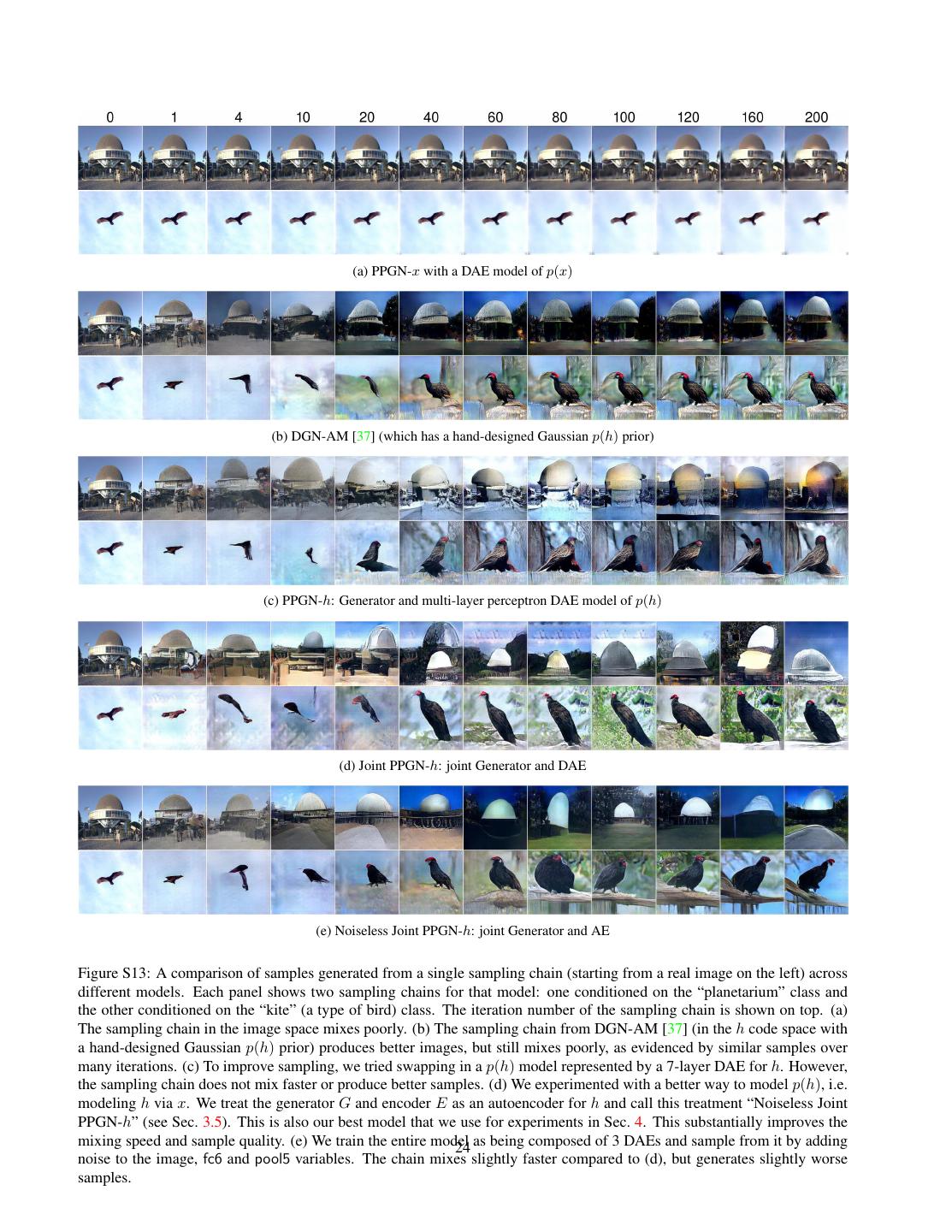
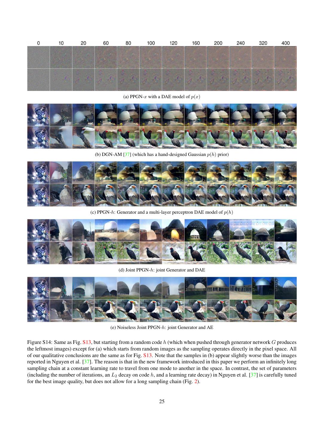
5 . ∂ log p(y = yc |xt ) p(h, y) = p(h)p(y|h) (9) xt+1 = xt + 1 Rx (xt )−xt + 2 +N (0, 23 ) ∂xt From Eq. 5, if we define a Gaussian p(h) centered at (7) 0 and set ( 1 , 2 , 3 ) = (λ, 1, 0), pulling Gaussian con- 3.1. PPGN-x: DAE model of p(x) stants into λ, we obtain the following noiseless update rule in Nguyen et al. [37] to sample h from class yc : First, we tested using a DAE to model p(x) directly (Fig. 3a) and sampling from the entire model via Eq. 7. ∂ log p(y = yc |ht ) ht+1 = (1 − λ)ht + 2 However, we found that PPGN-x exhibits two expected ∂ht problems: (1) it models the data distribution poorly; and ∂ log Cc (G(ht )) ∂G(ht ) (2) the chain mixes slowly. More details are in Sec. S11. = (1 − λ)ht + 2 (10) ∂G(ht ) ∂ht 3.2. DGN-AM: sampling without a learned prior where Cc (·) represents the output unit associated with class Poor mixing in the high-dimensional pixel space of yc . As before, all terms are computable in a single forward- PPGN-x is consistent with previous observations that mix- backward pass. More concretely, to compute the 2 term, ing on higher layers can result in faster exploration of the we push a code h through the generator G and condition space [5, 33]. Thus, to ameliorate the problem of slow network C to the output class c that we want to condition mixing, we may reparameterize p(x) as h p(h)p(x|h)dh on (Fig. 3b, red arrows), and back-propagate the gradient for some latent h, and perform sampling in this lower- via the same path to h. The final h is pushed through G to dimensional h-space. produce an image sample. While several recent works had success with this ap- Under this newly proposed framework, we have success- proach [37, 6, 63], they often hand-design the p(h) prior. fully reproduced the original DGN-AM results and their is- Among these, the DGN-AM method [37] searches in the sue of converging to the same mode when starting from dif- latent space of a generator network G to find a code h such ferent random initializations (Fig. 2b). We also found that that the image G(h) highly activates a given neuron in a tar- DGN-AM mixes somewhat poorly, yielding the same image get DNN. We start by reproducing their results for compari- after many sampling steps (Figs. S13b & S14b). son. G is trained following the methodology in Dosovitskiy & Brox [9] with an L2 image reconstruction loss, a Genera- 3.3. PPGN-h: Generator and DAE model of p(h) tive Adversarial Networks (GAN) loss [14], and an L2 loss We attempt to address the poor mixing speed of DGN- in a feature space h1 of an encoder E (Fig. 3f). The last loss AM by incorporating a proper p(h) prior learned via a DAE encourages generated images to match the real images in a into the sampling procedure described in Sec. 3.2. Specifi- high-level feature space and is referred to as “feature match- cally, we train Rh , a 7-layer, fully-connected DAE on h (as ing” [47] in this paper, but is also known as “perceptual sim- before, h is a fc6 feature vector). The size of the hidden lay- ilarity” [28, 9] or a form of “moment matching” [31]. Note ers are respectively: 4096 − 2048 − 1024 − 500 − 1024 − that in the GAN training for G, we simultaneously train a 2048 − 4096. Full training details are provided in S9.3. discriminator D to tell apart real images x vs. generated The update rule to sample h from this model is similar to images G(h). More training details are in Sec. S9.4. Eq. 10 except for the inclusion of all three terms: The directed graphical model interpretation of DGN-AM is h → x → y (see Fig. 3b) and the joint p(h, x, y) can be ∂ log Cc (G(ht )) ∂G(ht ) ht+1 = ht + 1 (Rh (ht )−ht )+ 2 decomposed into: ∂G(ht ) ∂ht 2 +N (0, 3) (11) p(h, x, y) = p(h)p(x|h)p(y|x) (8) where h in this case represents features extracted from Concretely, to compute Rh (ht ) we push ht through the the first fully connected layer (called fc6) of a pre-trained learned DAE, encoding and decoding it (Fig. 3c, black ar- AlexNet [26] 1000-class ImageNet [7] classification net- rows). The 2 term is computed via a forward and backward work (see Fig. 3f). p(x|h) is modeled by G, an upconvolu- pass through both G and C networks as before (Fig. 3c, red tional (also “deconvolutional”) network [10] with 9 upcon- arrows). Lastly, we add the same amount of noise N (0, 23 ) volutional and 3 fully connected layers. p(y|x) is modeled used during DAE training to h. Equivalently, noise can also by C, which in this case is also the AlexNet classifier. The be added before the encode-decode step. model for p(h) was an implicit unimodal Gaussian imple- We sample4 using ( 1 , 2 , 3 ) = (10−5 , 1, 10−5 ) and mented via L2 decay in h-space [37]. show results in Figs. S13c & S14c. As expected, the chain Since x is a deterministic variable, the model simplifies 4 If faster mixing or more stable samples are desired, then 1 and 3 to: can be scaled up or down together. Here we scale both down to 10−5 . 5 

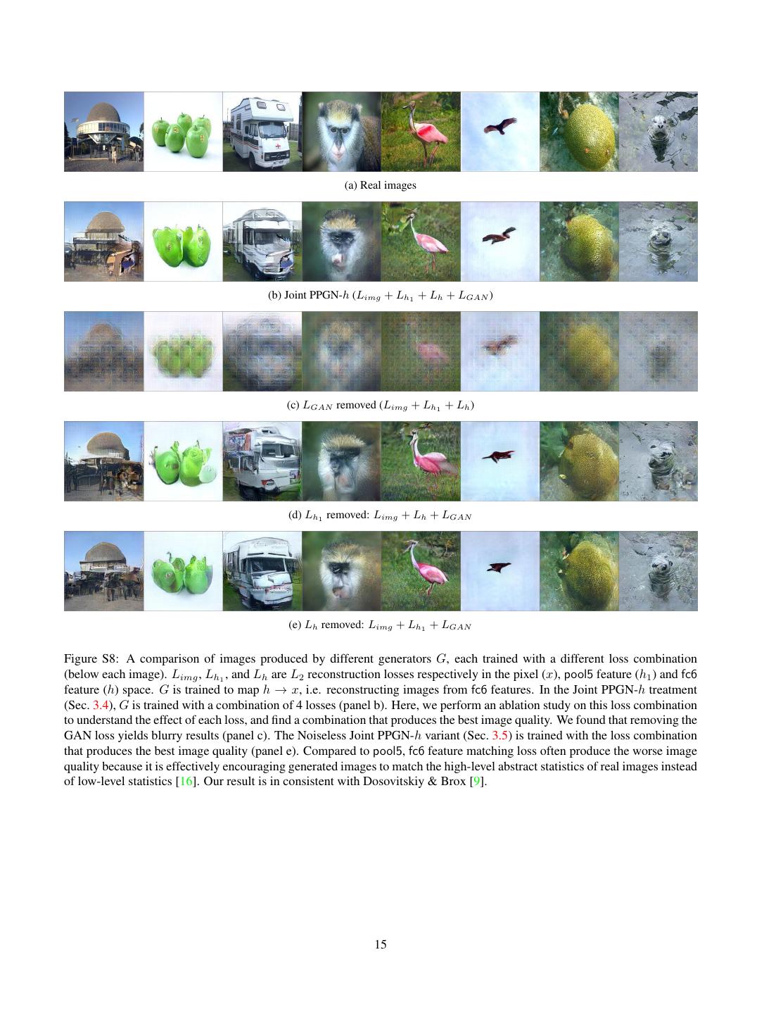
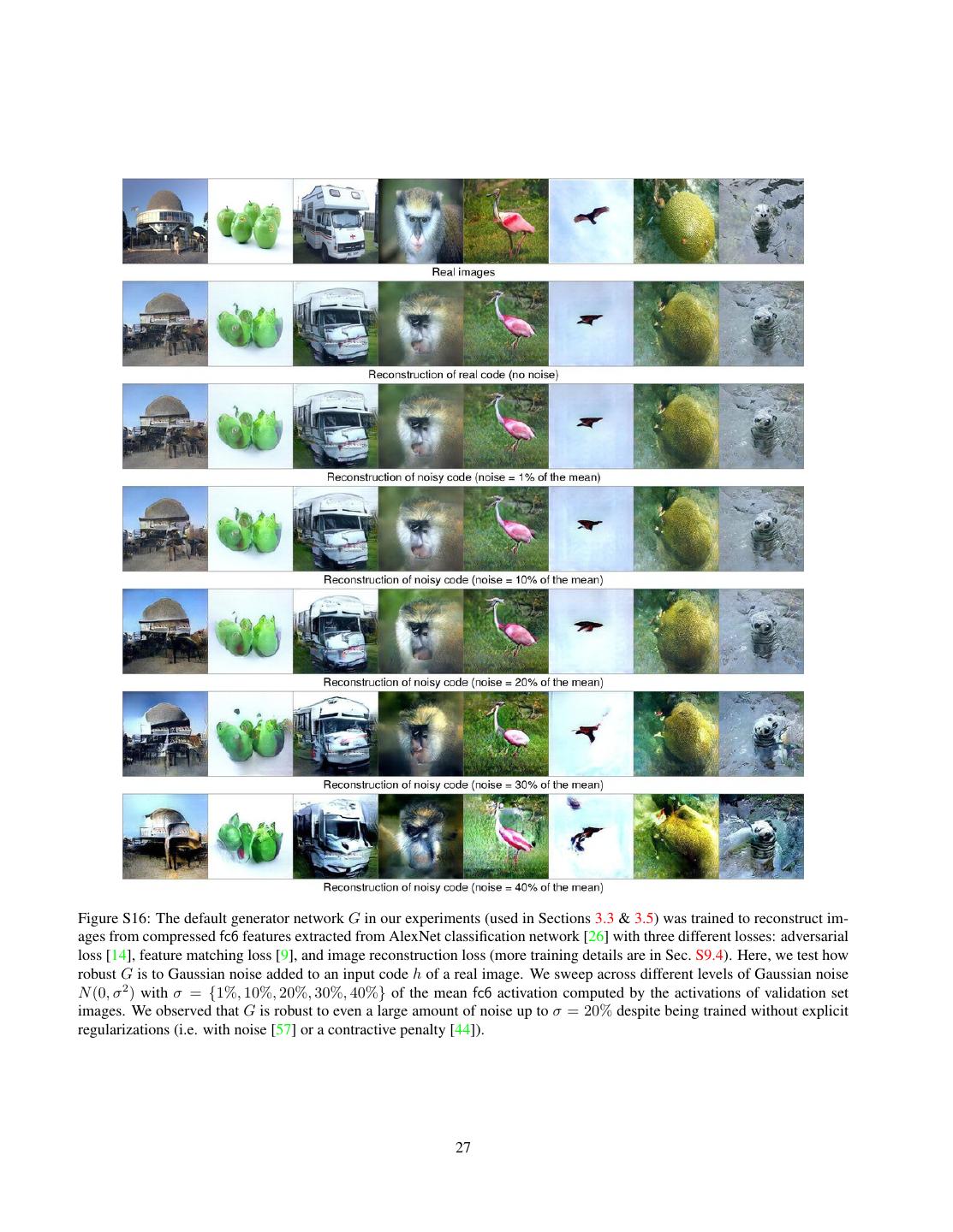
6 .mixes faster than PPGN-x, with subsequent samples ap- ing process can be difficult to understand, making further pearing more qualitatively different from their predecessors. improvements non-intuitive. To shed more light into how However, the samples for PPGN-h are qualitatively similar the Joint PPGN-h works, we perform ablation experiments to those from DGN-AM (Figs. S13b & S14b). Samples still which later reveal a better-performing variant. lack quality and diversity, which we hypothesize is due to Noise sweeps. To understand the effects of adding noise the poor p(h) model learned by the DAE. to each variable, we train variants of the Joint PPGN-h (1) with different noise levels, (2) using noise on only a single 3.4. Joint PPGN-h: joint Generator and DAE variable, and (3) using noise on multiple variables simulta- The previous result suggests that the simple multi-layer neously. We did not find these variants to produce qualita- perceptron DAE poorly modeled the distribution of fc6 fea- tively better reconstruction results than the Joint PPGN-h. tures. This could occur because the DAE faces the gener- Interestingly, in a PPGN variant trained with no noise at all, ally difficult unconstrained density estimation problem. To the h-autoencoder given by G(E(.)) still appears to be con- combat this issue, we experiment with modeling h via x tractive, i.e. robust to a large amount of noise (Fig. S16). with a DAE: h → x → h. Intuitively, to help the DAE bet- This is beneficial during sampling; if “unrealistic” codes ter model h, we force it to generate realistic-looking images appear, G could map them back to realistic-looking im- x from features h and then decode them back to h. One can ages. We believe this property might emerge for multiple train this DAE from scratch separately from G (as done for reasons: (1) G and E are not trained jointly; (2) h features PPGN-h). However, in the DGN-AM formulation, G mod- encode global, high-level rather than local, low-level infor- els the h → x (Fig. 3b) and E models the x → h (Fig. 3f). mation; (3) the presence of the adversarial cost when train- Thus, the composition G(E(.)) can be considered an AE ing G could make the h → x mapping more “many-to-one” h → x → h (Fig. 3d). by pushing x towards modes of the image distribution. Note that G(E(.)) is theoretically not a formal h-DAE Combinations of losses. To understand the effects of because its two components were trained with neither noise each loss component, we repeat the Joint PPGN-h training added to h nor an L2 reconstruction loss for h [37] (more (Sec. 3.4), but without noise added to the variables. Specif- details in Sec. S9.4) as is required for regular DAE train- ically, we test different combinations of losses and compare ing [57]. To make G(E(.)) a more theoretically justifiable the quality of images G(h) produced by pushing the codes h-DAE, we add noise to h and train G with an additional re- h of real images through G (without MCMC sampling). construction loss for h (Fig. S9c). We do the same for x and First, we found that removing the adversarial loss from h1 (pool5 features), hypothesizing that a little noise added the 4-loss combination yields blurrier images (Fig. S8c). to x and h1 might encourage G to be more robust [57]. In Second, we compare 3 different feature matching losses: other words, with the same existing network structures from fc6, pool5, and both fc6 and pool5 combined, and found DGN-AM [37], we train G differently by treating the entire that pool5 feature matching loss leads to the best image model as being composed of 3 interleaved DAEs that share quality (Sec. S8). Our result is consistent with Dosovitskiy parameters: one each for h, h1 , and x (see Fig. S9c). Note & Brox [9]. Thus, the model that we found empirically to that E remains frozen, and G is trained with 4 losses in to- produce the best image quality is trained without noise and tal i.e. three L2 reconstruction losses for x, h, and h1 and a with three losses: a pool5 feature matching loss, an adver- GAN loss for x. See Sec. S9.5 for full training details. We sarial loss, and an image reconstruction loss. We call this call this the Joint PPGN-h model. variant “Noiseless Joint PPGN-h”: it produced the results We sample from this model following the update rule in in Figs. 1 & 2 and Sections 3.5 & 4. Eq. 11 with ( 1 , 2 ) = (10−5 , 1), and with noise added to Noiseless Joint PPGN-h. We sample from this model all three variables: h, h1 and x instead of only to h (Fig. 3d with ( 1 , 2 , 3 ) = (10−5 , 1, 10−17 ) following the same up- vs e). The noise amounts added at each layer are the same date rule in Eq. 11 (we need noise to make it a proper sam- as those used during training. As hypothesized, we observe pling procedure, but found that infinitesimally small noise that the sampling chain from this model mixes substan- produces better and more diverse images, which is to be tially faster and produces samples with better quality than expected given that the DAE in this variant was trained all previous PPGN treatments (Figs. S13d & S14d) includ- without noise). Interestingly, the chain mixes substantially ing PPGN-h, which has a multi-layer perceptron h-DAE. faster than DGN-AM (Figs. S13e & S13b) although the only difference between two treatments is the existence of 3.5. Ablation study with Noiseless Joint PPGN-h the learned p(h) prior. Overall, the Noiseless Joint PPGN- While the Joint PPGN-h outperforms all previous treat- h produces a large amount of sample diversity (Fig. 2). ments in sample quality and diversity (as the chain mixes Compared to the Joint PPGN-h, the Noiseless Joint PPGN- faster), the model is trained with a combination of four h produces better image quality, but mixes slightly slower losses and noise added to all variables. This complex train- (Figs. S13 & S14). Sweeping across the noise levels dur- 6 

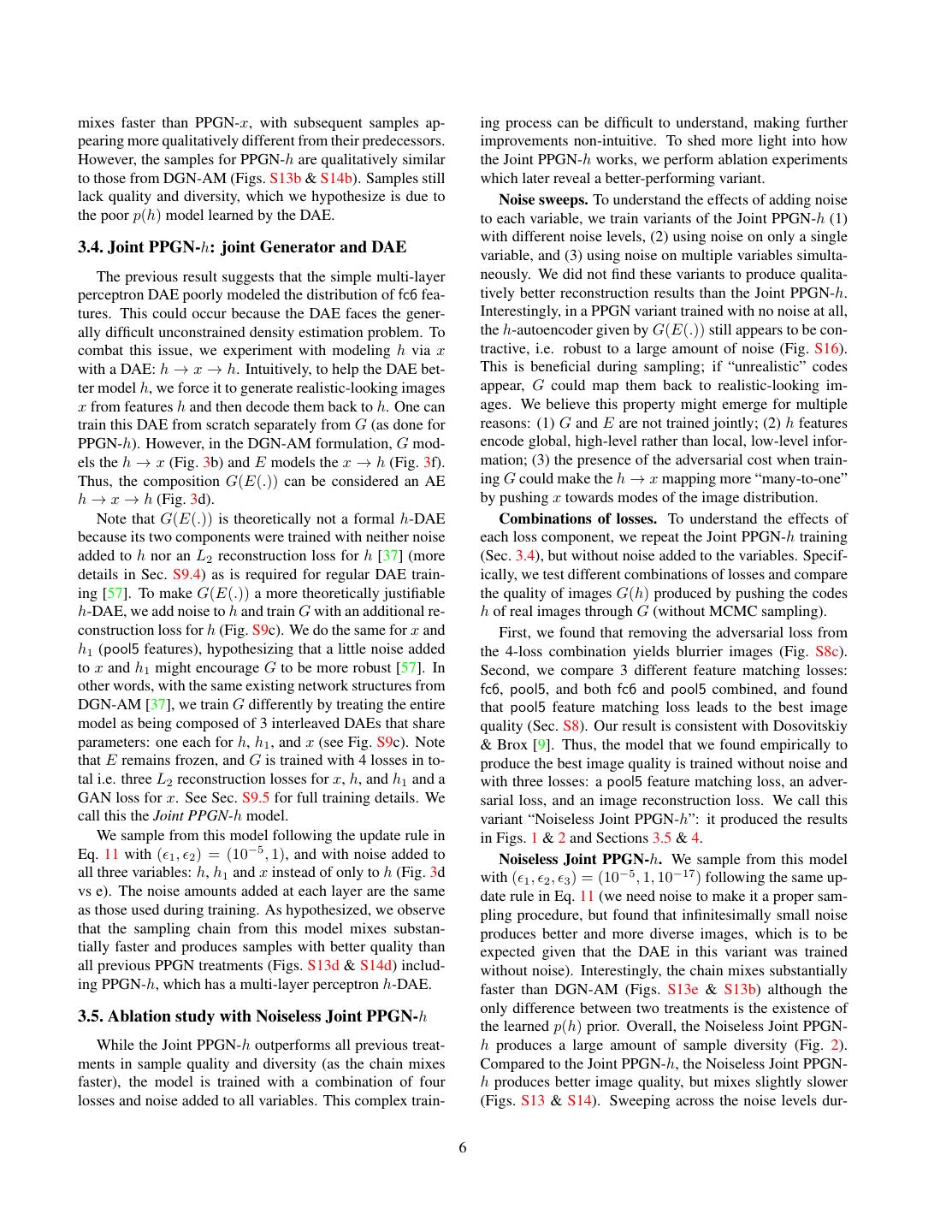
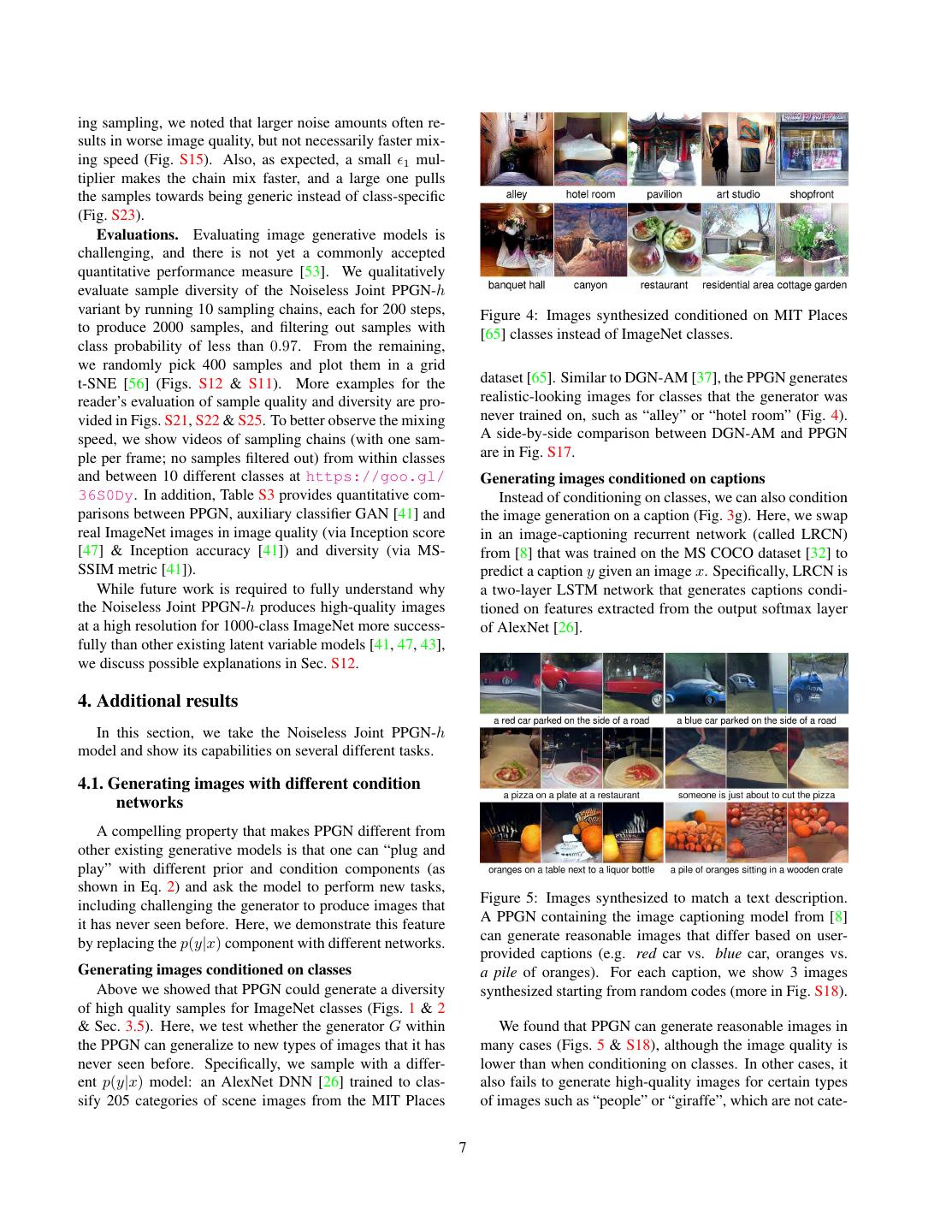
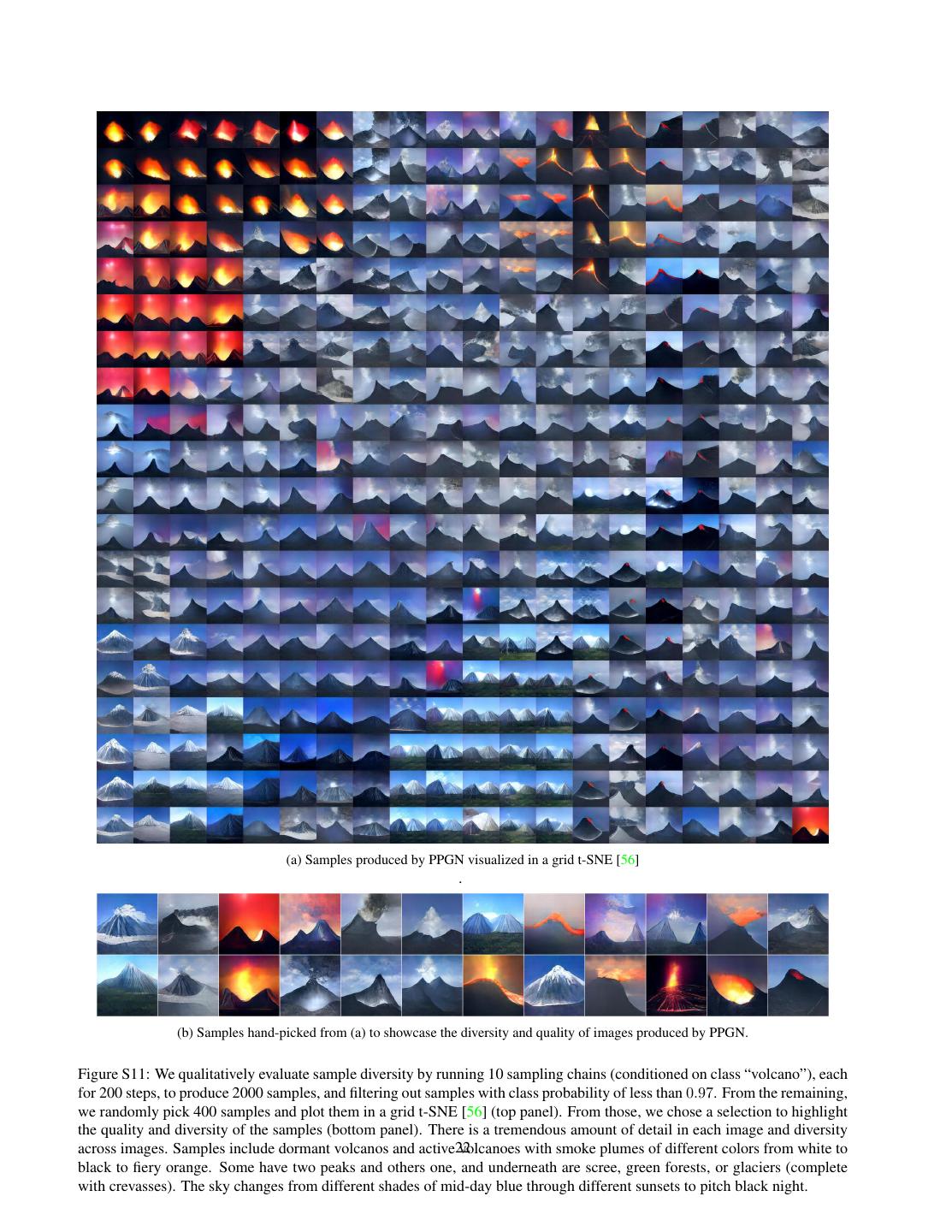
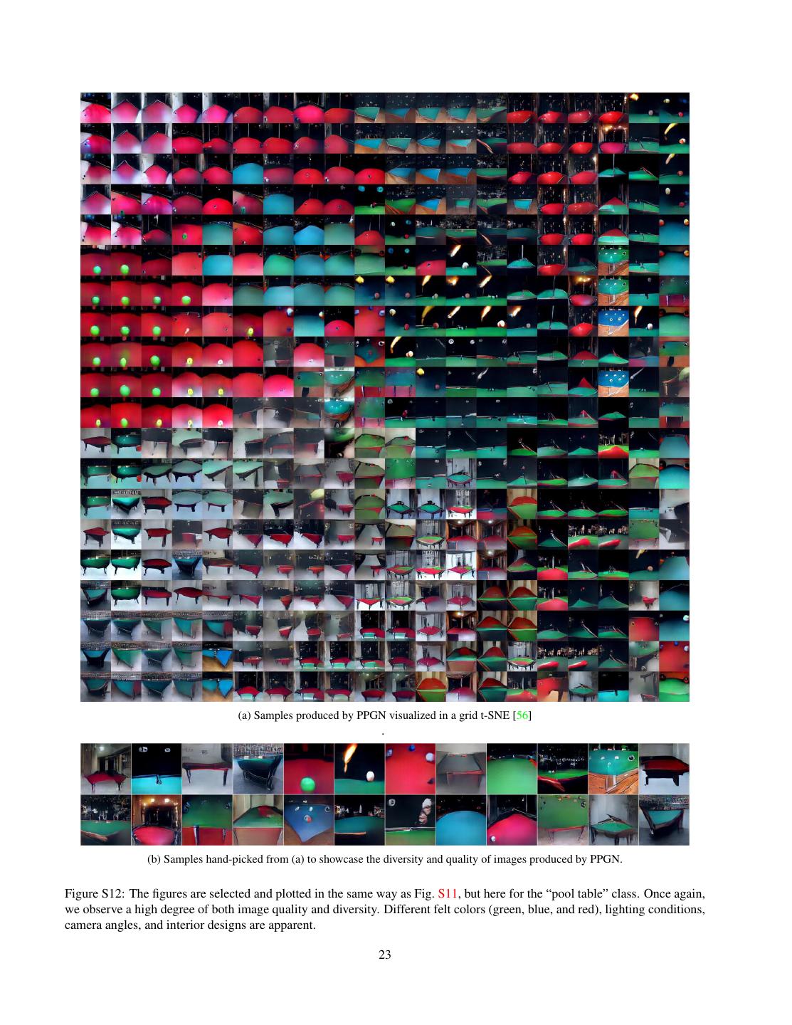
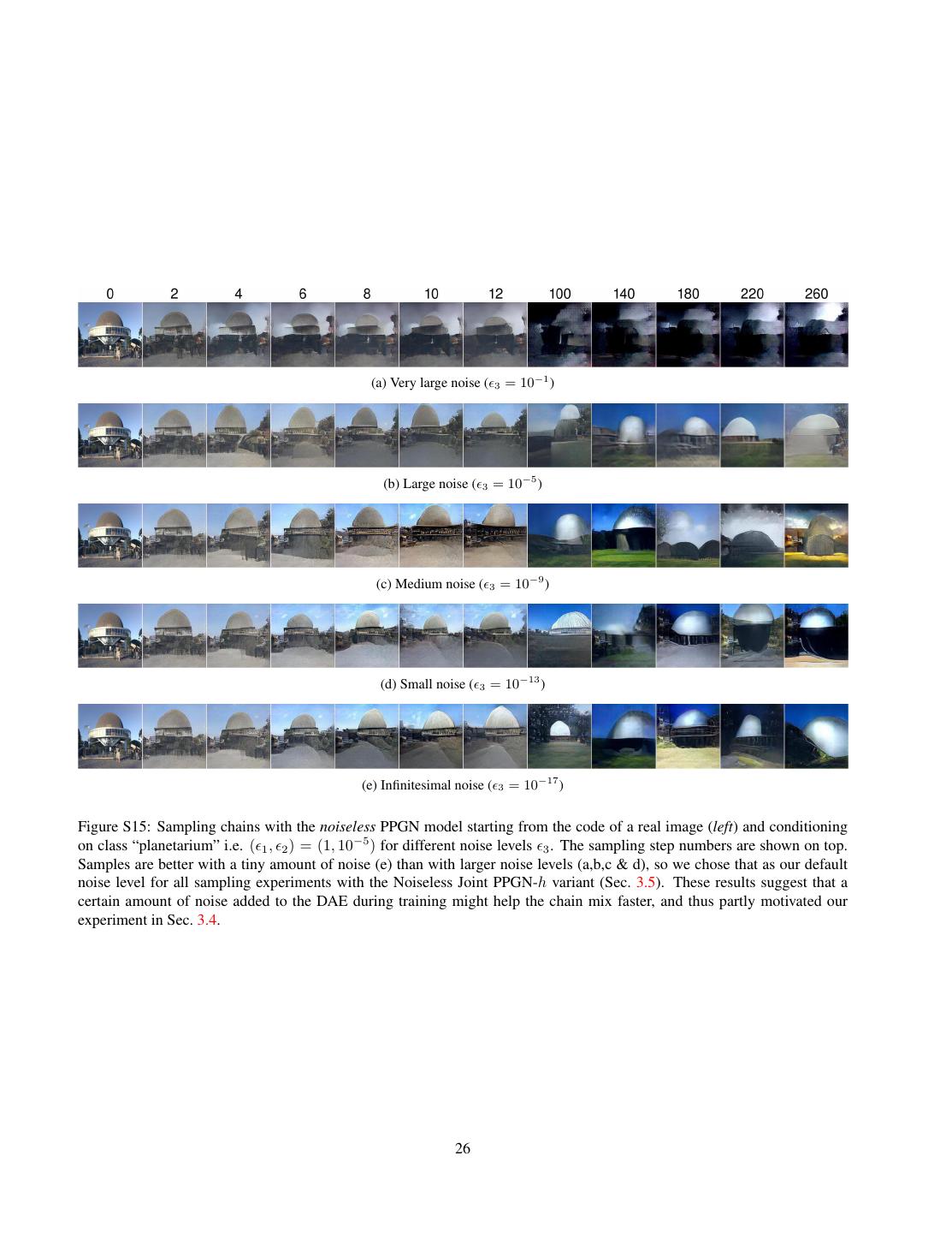
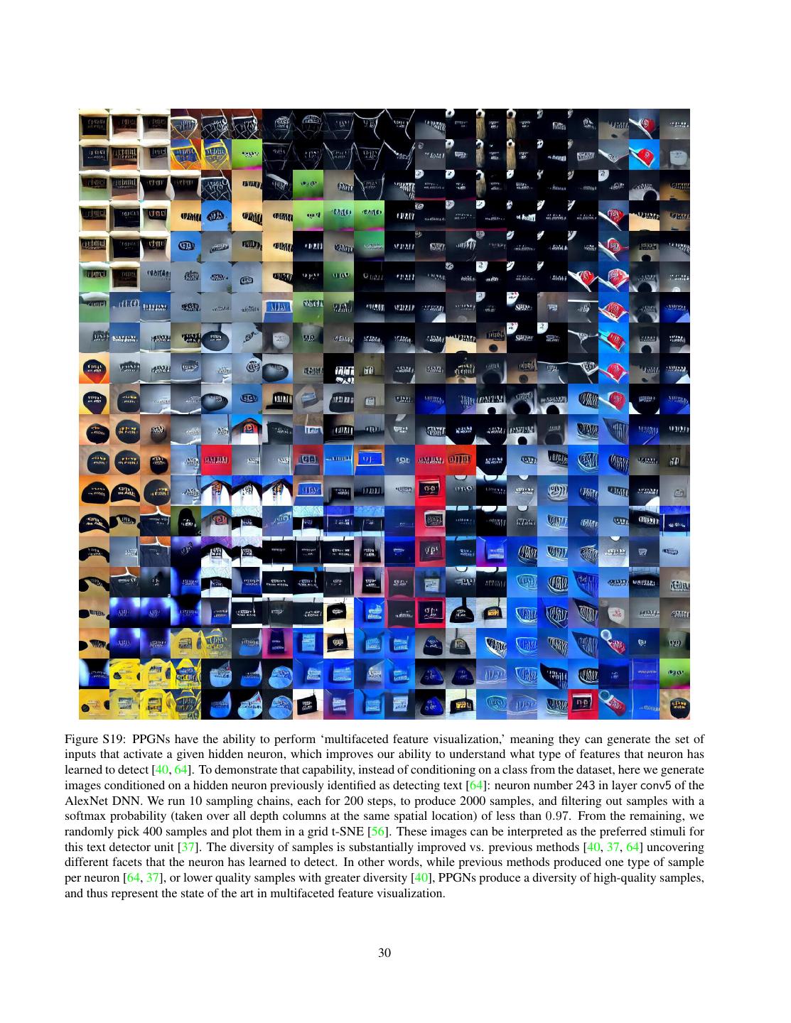
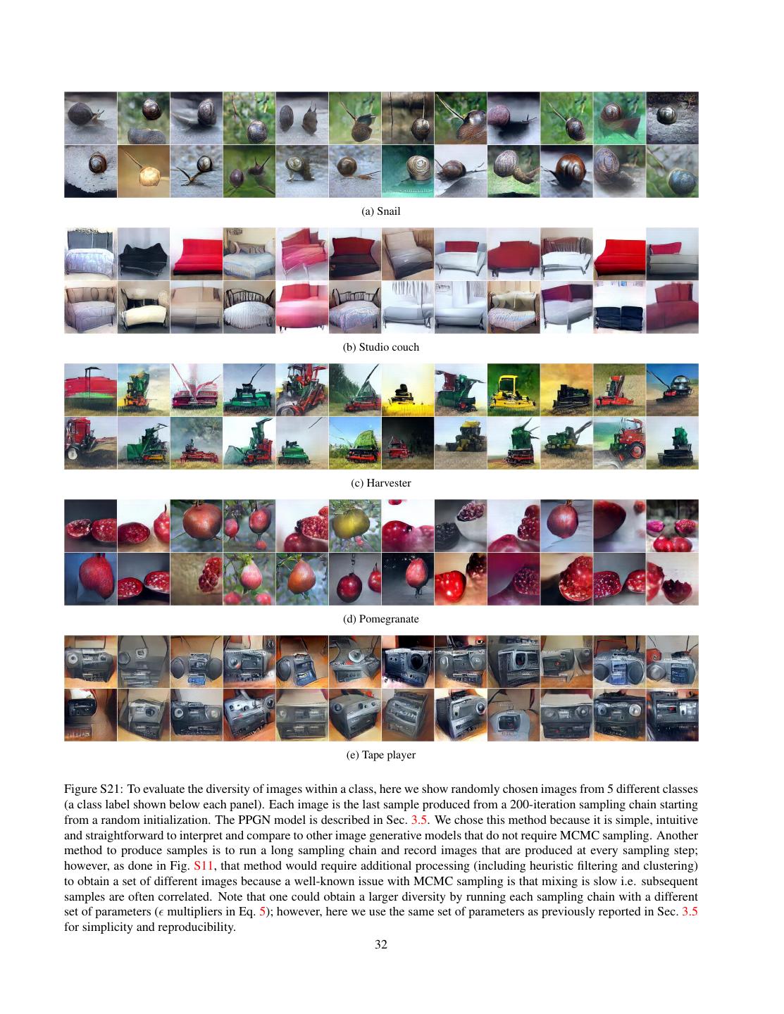
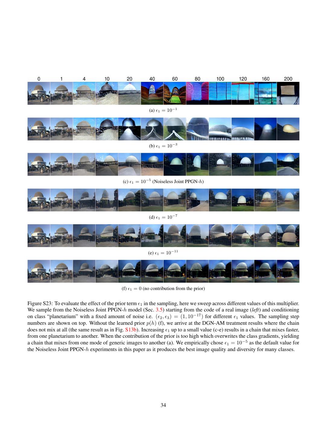
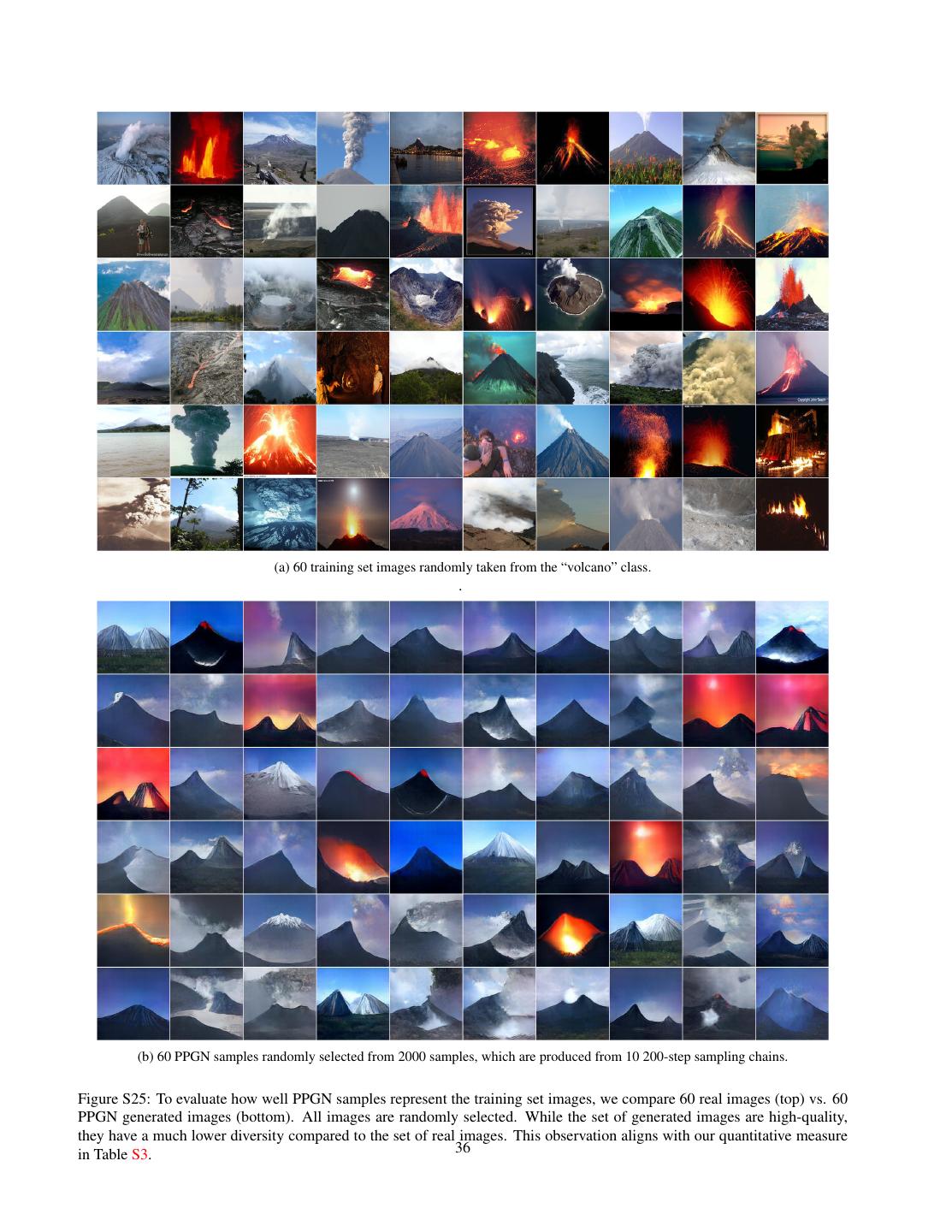
7 .ing sampling, we noted that larger noise amounts often re- sults in worse image quality, but not necessarily faster mix- ing speed (Fig. S15). Also, as expected, a small 1 mul- tiplier makes the chain mix faster, and a large one pulls the samples towards being generic instead of class-specific (Fig. S23). Evaluations. Evaluating image generative models is challenging, and there is not yet a commonly accepted quantitative performance measure [53]. We qualitatively evaluate sample diversity of the Noiseless Joint PPGN-h variant by running 10 sampling chains, each for 200 steps, Figure 4: Images synthesized conditioned on MIT Places to produce 2000 samples, and filtering out samples with [65] classes instead of ImageNet classes. class probability of less than 0.97. From the remaining, we randomly pick 400 samples and plot them in a grid t-SNE [56] (Figs. S12 & S11). More examples for the dataset [65]. Similar to DGN-AM [37], the PPGN generates reader’s evaluation of sample quality and diversity are pro- realistic-looking images for classes that the generator was vided in Figs. S21, S22 & S25. To better observe the mixing never trained on, such as “alley” or “hotel room” (Fig. 4). speed, we show videos of sampling chains (with one sam- A side-by-side comparison between DGN-AM and PPGN ple per frame; no samples filtered out) from within classes are in Fig. S17. and between 10 different classes at https://goo.gl/ Generating images conditioned on captions 36S0Dy. In addition, Table S3 provides quantitative com- Instead of conditioning on classes, we can also condition parisons between PPGN, auxiliary classifier GAN [41] and the image generation on a caption (Fig. 3g). Here, we swap real ImageNet images in image quality (via Inception score in an image-captioning recurrent network (called LRCN) [47] & Inception accuracy [41]) and diversity (via MS- from [8] that was trained on the MS COCO dataset [32] to SSIM metric [41]). predict a caption y given an image x. Specifically, LRCN is While future work is required to fully understand why a two-layer LSTM network that generates captions condi- the Noiseless Joint PPGN-h produces high-quality images tioned on features extracted from the output softmax layer at a high resolution for 1000-class ImageNet more success- of AlexNet [26]. fully than other existing latent variable models [41, 47, 43], we discuss possible explanations in Sec. S12. 4. Additional results In this section, we take the Noiseless Joint PPGN-h model and show its capabilities on several different tasks. 4.1. Generating images with different condition networks A compelling property that makes PPGN different from other existing generative models is that one can “plug and play” with different prior and condition components (as shown in Eq. 2) and ask the model to perform new tasks, Figure 5: Images synthesized to match a text description. including challenging the generator to produce images that A PPGN containing the image captioning model from [8] it has never seen before. Here, we demonstrate this feature can generate reasonable images that differ based on user- by replacing the p(y|x) component with different networks. provided captions (e.g. red car vs. blue car, oranges vs. Generating images conditioned on classes a pile of oranges). For each caption, we show 3 images Above we showed that PPGN could generate a diversity synthesized starting from random codes (more in Fig. S18). of high quality samples for ImageNet classes (Figs. 1 & 2 & Sec. 3.5). Here, we test whether the generator G within We found that PPGN can generate reasonable images in the PPGN can generalize to new types of images that it has many cases (Figs. 5 & S18), although the image quality is never seen before. Specifically, we sample with a differ- lower than when conditioning on classes. In other cases, it ent p(y|x) model: an AlexNet DNN [26] trained to clas- also fails to generate high-quality images for certain types sify 205 categories of scene images from the MIT Places of images such as “people” or “giraffe”, which are not cate- 7 

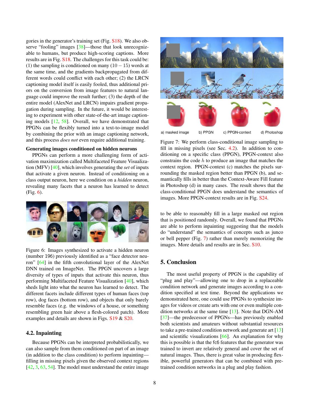
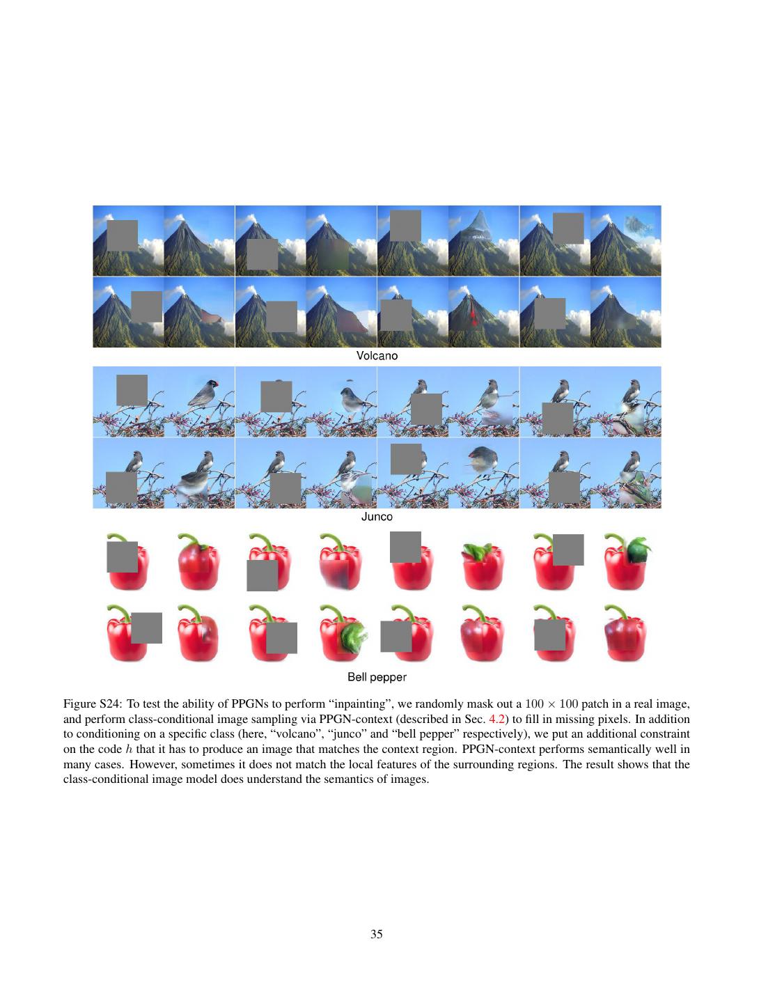
8 .gories in the generator’s training set (Fig. S18). We also ob- serve “fooling” images [38]—those that look unrecogniz- able to humans, but produce high-scoring captions. More results are in Fig. S18. The challenges for this task could be: (1) the sampling is conditioned on many (10 − 15) words at the same time, and the gradients backpropagated from dif- ferent words could conflict with each other; (2) the LRCN captioning model itself is easily fooled, thus additional pri- ors on the conversion from image features to natural lan- guage could improve the result further; (3) the depth of the entire model (AlexNet and LRCN) impairs gradient propa- gation during sampling. In the future, it would be interest- ing to experiment with other state-of-the-art image caption- ing models [12, 58]. Overall, we have demonstrated that PPGNs can be flexibly turned into a text-to-image model by combining the prior with an image captioning network, and this process does not even require additional training. Figure 7: We perform class-conditional image sampling to Generating images conditioned on hidden neurons fill in missing pixels (see Sec. 4.2). In addition to con- PPGNs can perform a more challenging form of acti- ditioning on a specific class (PPGN), PPGN-context also vation maximization called Multifaceted Feature Visualiza- constrains the code h to produce an image that matches the tion (MFV) [40], which involves generating the set of inputs context region. PPGN-context (c) matches the pixels sur- that activate a given neuron. Instead of conditioning on a rounding the masked region better than PPGN (b), and se- class output neuron, here we condition on a hidden neuron, mantically fills in better than the Context-Aware Fill feature revealing many facets that a neuron has learned to detect in Photoshop (d) in many cases. The result shows that the (Fig. 6). class-conditional PPGN does understand the semantics of images. More PPGN-context results are in Fig. S24. to be able to reasonably fill in a large masked out region that is positioned randomly. Overall, we found that PPGNs are able to perform inpainting suggesting that the models do “understand” the semantics of concepts such as junco or bell pepper (Fig. 7) rather than merely memorizing the images. More details and results are in Sec. S10. Figure 6: Images synthesized to activate a hidden neuron (number 196) previously identified as a “face detector neu- ron” [64] in the fifth convolutional layer of the AlexNet 5. Conclusion DNN trained on ImageNet. The PPGN uncovers a large diversity of types of inputs that activate this neuron, thus The most useful property of PPGN is the capability of performing Multifaceted Feature Visualization [40], which “plug and play”—allowing one to drop in a replaceable sheds light into what the neuron has learned to detect. The condition network and generate images according to a con- different facets include different types of human faces (top dition specified at test time. Beyond the applications we row), dog faces (bottom row), and objects that only barely demonstrated here, one could use PPGNs to synthesize im- resemble faces (e.g. the windows of a house, or something ages for videos or create arts with one or even multiple con- resembling green hair above a flesh-colored patch). More dition networks at the same time [13]. Note that DGN-AM examples and details are shown in Figs. S19 & S20. [37]—the predecessor of PPGNs—has previously enabled both scientists and amateurs without substantial resources to take a pre-trained condition network and generate art [13] 4.2. Inpainting and scientific visualizations [66]. An explanation for why Because PPGNs can be interpreted probabilistically, we this is possible is that the fc6 features that the generator was can also sample from them conditioned on part of an image trained to invert are relatively general and cover the set of (in addition to the class condition) to perform inpainting— natural images. Thus, there is great value in producing flex- filling in missing pixels given the observed context regions ible, powerful generators that can be combined with pre- [42, 3, 63, 54]. The model must understand the entire image trained condition networks in a plug and play fashion. 8 

9 .Acknowledgments [13] G. Goh. Image synthesis from yahoo open nsfw. https: //opennsfw.gitlab.io, 2016. 2, 8 We thank Theo Karaletsos and Noah Goodman for help- [14] I. Goodfellow, J. Pouget-Abadie, M. Mirza, B. Xu, ful discussions, and Jeff Donahue for providing a trained D. Warde-Farley, S. Ozair, A. Courville, and Y. Bengio. Gen- image captioning model [8] for our experiments. We also erative adversarial nets. In Advances in Neural Information thank Joost Huizinga, Christopher Stanton, Rosanne Liu, Processing Systems, pages 2672–2680, 2014. 2, 5, 16, 18, Tyler Jaszkowiak, Richard Yang, and Jon Berliner for in- 19, 27 valuable suggestions on preliminary drafts. [15] K. Gregor, I. Danihelka, A. Graves, and D. Wierstra. Draw: A recurrent neural network for image generation. In ICML, References 2015. 1 [16] A. Gretton, K. M. Borgwardt, M. Rasch, B. Sch¨olkopf, and [1] G. Alain and Y. Bengio. What regularized auto-encoders A. J. Smola. A kernel method for the two-sample-problem. learn from the data-generating distribution. The Journal of In Advances in neural information processing systems, pages Machine Learning Research, 15(1):3563–3593, 2014. 4, 17, 513–520, 2006. 15 19 [2] K. Arulkumaran, A. Creswell, and A. A. Bharath. Improving [17] T. Han, Y. Lu, S.-C. Zhu, and Y. N. Wu. Alternating back- sampling from generative autoencoders with markov chains. propagation for generator network. In AAAI, 2017. 3, 13 arXiv preprint arXiv:1610.09296, 2016. 3, 13 [18] W. K. Hastings. Monte carlo sampling methods using [3] C. Barnes, E. Shechtman, A. Finkelstein, and D. Goldman. markov chains and their applications. Biometrika, 57(1):97– Patchmatch: a randomized correspondence algorithm for 109, 1970. 12 structural image editing. ACM Transactions on Graphics- [19] G. E. Hinton. Products of experts. In Artificial Neural Net- TOG, 28(3):24, 2009. 8, 17 works, 1999. ICANN 99. Ninth International Conference on [4] I. G. Y. Bengio and A. Courville. Deep learning. Book in (Conf. Publ. No. 470), volume 1, pages 1–6. IET, 1999. 3 preparation for MIT Press, 2016. 2, 12 [20] S. Ioffe and C. Szegedy. Batch normalization: Accelerating [5] Y. Bengio, G. Mesnil, Y. Dauphin, and S. Rifai. Better mix- deep network training by reducing internal covariate shift. ing via deep representations. In Proceedings of the 30th In- In Proceedings of the 32nd International Conference on Ma- ternational Conference on Machine Learning (ICML), pages chine Learning, ICML 2015, Lille, France, 6-11 July 2015, 552–560, 2013. 5 2015. 16 [6] A. Brock, T. Lim, J. Ritchie, and N. Weston. Neural [21] Y. Jia. Caffe: An open source convolutional archi- photo editing with introspective adversarial networks. arXiv tecture for fast feature embedding. http://caffe. preprint arXiv:1609.07093, 2016. 3, 5, 13 berkeleyvision.org/, 2013. 16 [7] J. Deng, W. Dong, R. Socher, L.-J. Li, K. Li, and L. Fei- [22] J. Johnson, A. Alahi, and L. Fei-Fei. Perceptual losses for Fei. Imagenet: A large-scale hierarchical image database. real-time style transfer and super-resolution. arXiv preprint In Computer Vision and Pattern Recognition, 2009. CVPR arXiv:1603.08155, 2016. 14 2009. IEEE Conference on, pages 248–255. IEEE, 2009. 2, [23] D. Kingma and J. Ba. Adam: A method for stochastic opti- 5, 14, 16, 29 mization. arXiv preprint arXiv:1412.6980, 2014. 16 [8] J. Donahue, L. A. Hendricks, S. Guadarrama, M. Rohrbach, [24] D. P. Kingma and M. Welling. Auto-Encoding Variational S. Venugopalan, K. Saenko, and T. Darrell. Long-term re- Bayes. Dec. 2014. 1, 19 current convolutional networks for visual recognition and [25] D. Koller and N. Friedman. Probabilistic graphical models: description. In Computer Vision and Pattern Recognition, principles and techniques. MIT press, 2009. 3, 12 2015. 7, 9, 29 [26] A. Krizhevsky, I. Sutskever, and G. Hinton. Imagenet clas- [9] A. Dosovitskiy and T. Brox. Generating Images with Per- sification with deep convolutional neural networks. In Ad- ceptual Similarity Metrics based on Deep Networks. In Ad- vances in Neural Information Processing Systems 25, pages vances in Neural Information Processing Systems, 2016. 1, 1106–1114, 2012. 3, 5, 7, 14, 16, 18, 27 5, 6, 14, 15, 16, 18, 27 [10] A. Dosovitskiy, J. Tobias Springenberg, and T. Brox. Learn- [27] H. Larochelle and I. Murray. The neural autoregressive dis- ing to generate chairs with convolutional neural networks. tribution estimator. Journal of Machine Learning Research, In Proceedings of the IEEE Conference on Computer Vision 15:29–37, 2011. 1 and Pattern Recognition, pages 1538–1546, 2015. 5, 16 [28] A. B. L. Larsen, S. K. Sønderby, and O. Winther. Autoencod- [11] D. Erhan, Y. Bengio, A. Courville, and P. Vincent. Visualiz- ing beyond pixels using a learned similarity metric. CoRR, ing higher-layer features of a deep network. Technical report, abs/1512.09300, 2015. 5, 14 Technical report, University of Montreal, 2009. 2, 3, 13, 14 [29] Y. LeCun, S. Chopra, R. Hadsell, M. Ranzato, and F. Huang. [12] A. Frome, G. S. Corrado, J. Shlens, S. Bengio, J. Dean, M. A. A tutorial on energy-based learning. Predicting structured Ranzato, and T. Mikolov. Devise: A deep visual-semantic data, 1:0, 2006. 2 embedding model. In C. Burges, L. Bottou, M. Welling, [30] C. Ledig, L. Theis, F. Husz´ar, J. Caballero, A. Aitken, A. Te- Z. Ghahramani, and K. Weinberger, editors, Advances in jani, J. Totz, Z. Wang, and W. Shi. Photo-realistic single im- Neural Information Processing Systems 26, pages 2121– age super-resolution using a generative adversarial network. 2129. Curran Associates, Inc., 2013. 8 arXiv preprint arXiv:1609.04802, 2016. 2 9 

10 .[31] Y. Li, K. Swersky, and R. Zemel. Generative moment [46] G. O. Roberts and R. L. Tweedie. Exponential convergence matching networks. In International Conference on Machine of langevin distributions and their discrete approximations. Learning, pages 1718–1727, 2015. 5 Bernoulli, pages 341–363, 1996. 3, 12 [32] T.-Y. Lin, M. Maire, S. Belongie, J. Hays, P. Perona, D. Ra- [47] T. Salimans, I. J. Goodfellow, W. Zaremba, V. Cheung, manan, P. Doll´ar, and C. L. Zitnick. Microsoft coco: Com- A. Radford, and X. Chen. Improved techniques for train- mon objects in context. In European Conference on Com- ing gans. CoRR, abs/1606.03498, 2016. 2, 5, 7, 16, 18, 19, puter Vision, pages 740–755. Springer, 2014. 7 20 [33] H. Luo, P. L. Carrier, A. C. Courville, and Y. Bengio. Texture [48] K. Simonyan, A. Vedaldi, and A. Zisserman. Deep inside modeling with convolutional spike-and-slab rbms and deep convolutional networks: Visualising image classification extensions. In AISTATS, pages 415–423, 2013. 5 models and saliency maps. arXiv preprint arXiv:1312.6034, [34] A. Mahendran and A. Vedaldi. Visualizing deep convolu- presented at ICLR Workshop 2014, 2013. 2, 3, 13, 14 tional neural networks using natural pre-images. Interna- [49] K. Simonyan and A. Zisserman. Very deep convolu- tional Journal of Computer Vision, pages 1–23, 2016. 3, 13, tional networks for large-scale image recognition. CoRR, 14 abs/1409.1556, 2014. 3 [35] N. Metropolis, A. W. Rosenbluth, M. N. Rosenbluth, A. H. [50] C. Szegedy, S. Ioffe, and V. Vanhoucke. Inception-v4, Teller, and E. Teller. Equation of state calculations by inception-resnet and the impact of residual connections on fast computing machines. The journal of chemical physics, learning. CoRR, abs/1602.07261, 2016. 20 21(6):1087–1092, 1953. 12 [51] C. Szegedy, W. Zaremba, I. Sutskever, J. Bruna, D. Erhan, [36] A. Mordvintsev, C. Olah, and M. Tyka. Inceptionism: Go- I. J. Goodfellow, and R. Fergus. Intriguing properties of neu- ing deeper into neural networks. Google Research Blog. Re- ral networks. CoRR, abs/1312.6199, 2013. 3, 4, 13 trieved June, 20, 2015. 14 [52] Y. W. Teh, A. H. Thiery, and S. J. Vollmer. Consistency and [37] A. Nguyen, A. Dosovitskiy, J. Yosinski, T. Brox, and fluctuations for stochastic gradient langevin dynamics. 2014. J. Clune. Synthesizing the preferred inputs for neurons in 12 neural networks via deep generator networks. In Advances [53] L. Theis, A. van den Oord, and M. Bethge. A note on the in Neural Information Processing Systems, 2016. 1, 2, 3, 4, evaluation of generative models. Nov 2016. International 5, 6, 7, 8, 13, 14, 16, 17, 21, 24, 25, 28, 30 Conference on Learning Representations. 2, 7, 19 [38] A. Nguyen, J. Yosinski, and J. Clune. Deep neural networks [54] A. van den Oord, N. Kalchbrenner, and K. Kavukcuoglu. are easily fooled: High confidence predictions for unrecog- Pixel Recurrent Neural Networks. ArXiv e-prints, Jan. 2016. nizable images. The IEEE Conference on Computer Vision 1, 2, 8 and Pattern Recognition (CVPR), June 2015. 3, 4, 8, 13 [55] A. van den Oord, N. Kalchbrenner, O. Vinyals, L. Espeholt, [39] A. Nguyen, J. Yosinski, and J. Clune. Innovation engines: A. Graves, and K. Kavukcuoglu. Conditional image genera- Automated creativity and improved stochastic optimization tion with pixelcnn decoders. CoRR, abs/1606.05328, 2016. via deep learning. In Proceedings of the Genetic and Evolu- 2 tionary Computation Conference (GECCO), 2015. 3, 13 [56] L. Van der Maaten and G. Hinton. Visualizing data using t- [40] A. Nguyen, J. Yosinski, and J. Clune. Multifaceted fea- sne. Journal of Machine Learning Research, 9(11), 2008. 7, ture visualization: Uncovering the different types of features 22, 23, 30 learned by each neuron in deep neural networks. In Visu- [57] P. Vincent, H. Larochelle, Y. Bengio, and P.-A. Manzagol. alization for Deep Learning Workshop, ICML conference, Extracting and composing robust features with denoising au- 2016. 1, 2, 3, 8, 13, 14, 30 toencoders. In Proceedings of the 25th international confer- [41] A. Odena, C. Olah, and J. Shlens. Conditional Image Syn- ence on Machine learning, pages 1096–1103. ACM, 2008. thesis With Auxiliary Classifier GANs. ArXiv e-prints, Oct. 4, 6, 17, 19, 27 2016. 2, 7, 18, 20 [58] O. Vinyals, A. Toshev, S. Bengio, and D. Erhan. Show [42] D. Pathak, P. Krahenbuhl, J. Donahue, T. Darrell, and A. A. and tell: A neural image caption generator. arXiv preprint Efros. Context encoders: Feature learning by inpainting. arXiv:1411.4555, 2014. 8 arXiv preprint arXiv:1604.07379, 2016. 8, 17 [59] D. Wei, B. Zhou, A. Torrabla, and W. Freeman. Under- [43] A. Radford, L. Metz, and S. Chintala. Unsupervised Repre- standing intra-class knowledge inside cnn. arXiv preprint sentation Learning with Deep Convolutional Generative Ad- arXiv:1507.02379, 2015. 2, 14 versarial Networks. Nov. 2015. 1, 2, 7, 16, 18 [60] D. Wei, B. Zhou, A. Torrabla, and W. Freeman. Under- [44] S. Rifai, P. Vincent, X. Muller, X. Glorot, and Y. Bengio. standing intra-class knowledge inside cnn. arXiv preprint Contractive auto-encoders: Explicit invariance during fea- arXiv:1507.02379, 2015. 3, 13 ture extraction. In Proceedings of the 28th international [61] M. Welling and Y. W. Teh. Bayesian learning via stochas- conference on machine learning (ICML-11), pages 833–840, tic gradient langevin dynamics. In Proceedings of the 28th 2011. 27 International Conference on Machine Learning (ICML-11), [45] G. O. Roberts and J. S. Rosenthal. Optimal scaling of dis- pages 681–688, 2011. 3, 12 crete approximations to langevin diffusions. Journal of the [62] J. Xie, Y. Lu, S.-C. Zhu, and Y. N. Wu. Cooperative train- Royal Statistical Society: Series B (Statistical Methodology), ing of descriptor and generator networks. arXiv preprint 60(1):255–268, 1998. 3, 12 arXiv:1609.09408, 2016. 17 10 

11 .[63] R. Yeh, C. Chen, T. Y. Lim, M. Hasegawa-Johnson, and M. N. Do. Semantic image inpainting with perceptual and contextual losses. arXiv preprint arXiv:1607.07539, 2016. 3, 5, 8, 13 [64] J. Yosinski, J. Clune, A. Nguyen, T. Fuchs, and H. Lipson. Understanding neural networks through deep visualization. In Deep Learning Workshop, International Conference on Machine Learning (ICML), 2015. 2, 3, 8, 13, 14, 17, 30, 31 [65] B. Zhou, A. Khosla, A. ` Lapedriza, A. Oliva, and A. Tor- ralba. Object detectors emerge in deep scene cnns. In In- ternational Conference on Learning Representations (ICLR), volume abs/1412.6856, 2014. 7, 28 [66] B. Zhou, A. Khosla, A. Lapedriza, A. Torralba, and A. Oliva. Places: An image database for deep scene understanding. arXiv preprint arXiv:1610.02055, 2016. 2, 8 [67] J.-Y. Zhu, P. Kr¨ahenb¨uhl, E. Shechtman, and A. A. Efros. Generative visual manipulation on the natural image mani- fold. In European Conference on Computer Vision, pages 597–613. Springer, 2016. 3, 13 11 

12 . Supplementary materials for: Plug & Play Generative Networks: Conditional Iterative Generation of Images in Latent Space S6. Markov chain Monte Carlo methods and where f (·) is the slightly more complex calculation of derivation of MALA-approx α, with the notable property that as the step size goes to 0, f (·) → 1. This sampler preferentially steps in the di- Assume a distribution p(x) that we wish to produce sam- rection of higher probability, which allows it to spend less ples from. For certain distributions with amenable structure time rejecting low probability proposals, but it still requires it may be possible to write down directly an independent computation of p(x) to calculate α. and identically distributed (IID) sampler, but in general this The stochastic gradient Langevin dynamics (SGLD) can be difficult. In such cases where IID samplers are not method [61, 52] was proposed to sidestep this troublesome readily available, we may instead resort to Markov Chain requirement by generating probability proposals that are Monte Carlo (MCMC) methods for sampling. Complete based on a small subset of the data only: by using stochas- discussions of this topic fill books [25, 4]. Here we briefly tic gradient descent plus noise, by skipping the accept-reject review the background that led to the sampler we propose. step, and by using decreasing step sizes. Inspired by SGLD, In cases where evaluation of p(x) is possible, we can we define an approximate sampler by assuming small step write down the Metropolis-Hastings (hereafter: MH) sam- size and doing away with the reject step (by accepting ev- pler for p(x) [35, 18]. It requires a choice of proposal dis- ery sample). The idea is that the stochasticity of SGD itself tribution q(x |x); for simplicity we consider (and later use) introduces an implicit noise: although the resulting update a simple Gaussian proposal distribution. Starting with an does not produce asymptotically unbiased samples, it does x0 from some initial distribution, the sampler takes steps if we also anneal the step size (or, equivalently, gradually according to a transition operator defined by the below rou- increase the minibatch size). tine, with N (0, σ 2 ) shorthand for a sample from that Gaus- While an accept ratio of 1 is only approached in the limit sian proposal distribution: as the step size goes to zero, in practice we empirically ob- serve that this approximation produces reasonable samples 1. xt+1 = xt + N (0, σ 2 ) even for moderate step sizes. This approximation leads to a 2. α = p(xt+1 )/p(xt ) sampler defined by the simple update rule: 3. if α < 1, reject sample xt+1 with probability 1 − α by xt+1 = xt + σ 2 /2∇ log p(xt ) + N (0, σ 2 ) (12) setting xt+1 = xt , else keep xt+1 As explained below, we propose to decouple the two step sizes for each of the above two terms after xt , with two In theory, sufficiently many steps of this simple sampling independent scaling factors to allow independently tuning rule produce samples for any computable p(x), but in prac- each ( 12 and 3 in Eq. 13). This variant makes sense when tice it has two problems: it mixes slowly, because steps are we consider that the stochasticity of SGD itself introduces small and uncorrelated in time, and it requires us to be able more noise, breaking the direct link between the amount of to compute p(x) to calculate α, which is often not possi- noise injected and the step size under Langevin dynamics. ble. A Metropolis-adjusted Langevin algorithm (hereafter: We note that p(x) ∝ exp(−Energy(x)), ∇ log p(xt ) MALA) [46, 45] addresses the first problem. This sampler is just the gradient of the energy (because the partition follows a slightly modified procedure: function does not depend on x) and that the scaling fac- tor (σ 2 /2 in the above equation) can be partially absorbed 1. xt+1 = xt + σ 2 /2∇ log p(xt ) + N (0, σ 2 ) when changing the temperature associated with energy, 2. α = f (xt , xt+1 , p(xt+1 ), p(xt )) since temperature is just a multiplicative scaling factor in the energy. Changing that link between the two terms is 3. if α < 1, reject sample xt+1 with probability 1 − α by thus equivalent to changing temperature because the incor- setting xt+1 = xt , else keep xt+1 rect scale factor can be absorbed in the energy as a change 12 

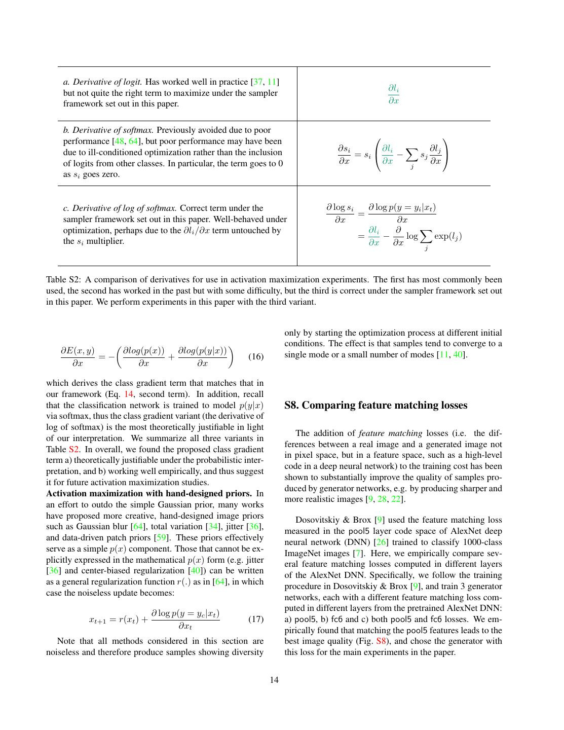
13 . uses accept/ reject step and mixes requires p(x) update rule (not including accept/reject step) MH slowly yes xt+1 = xt + N (0, σ 2 ) MALA ok yes xt+1 = xt + 1/2σ∇ log p(xt ) + N (0, σ 2 ) MALA-approx ok no xt+1 = xt + 12 ∇ log p(xt ) + N (0, 23 ) Table S1: Samplers properties assuming Gaussian proposal distributions. Samples are drawn via MALA-approx in this paper. in the temperature. Since we do not control directly the as a sampler with non-zero 1 but with a p(x) such that amount of noise (some of which is now produced by the ∂ log p(x) ∂x = 0; in other words, a uniform p(x) where all stochasticity of SGD itself), it is better to “manually” con- images are equally likely. trol the trade-off by introducing an extra hyperparameter. Activation maximization with a Gaussian prior. To com- Doing so also may help to compensate for the fact that the bat the fooling problem [38], several works have used L2 SGD noise is not perfectly normal, which introduces a bias decay, which can be thought of as a simple Gaussian prior in the Markov chain. By manually controlling both the step over images [48, 64, 60]. From Eq. 5, if we define a Gaus- size and the normal noise, we can thus find a good trade- sian p(x) centered at the origin (assume the mean image off between variance (or temperature level, which would has been subtracted) and set ( 1 , 2 , 3 ) = (λ, 1, 0), pulling blur the distribution) and bias (which makes us sample from Gaussian constants into λ, we obtain the following noiseless a slightly different distribution). In our experience, such update rule: decoupling has helped find better tradeoffs between sam- ple diversity and quality, perhaps compensating for idiosyn- ∂ log p(y = yc |xt ) xt+1 = (1 − λ)xt + (14) crasies of sampling without a reject step. We call this sam- ∂xt pler MALA-approx: The first term decays the current image slightly toward the origin, as appropriate under a Gaussian image prior, and 2 xt+1 = xt + 12 ∇ log p(xt ) + N (0, 3) (13) the second term pulls the image toward higher probability regions for the chosen class. Here, the second term is com- Table S1 summarizes the samplers and their properties. puted as the derivative of the log of a softmax unit in the output layer of the classification network, which is trained S7. Probabilistic interpretation of previous to model p(y|x). If we let li be the logit outputs of a classi- models (continued) fication network, where i indexes over the classes, then the In this paper, we consider four main representative ap- softmax outputs are given by si = exp(li )/ j exp(lj ), proaches in light of the framework: and the value p(y = yc |xt ) is modeled by the softmax unit sc . 1. Activation maximization with no priors [38, 51, 11] Note that the second term is similar, but not identical, to the gradient of logit term used by [48, 64, 34]. There 2. Activation maximization with a Gaussian prior [48, are three variants of computing this class gradient term: 1) 64] derivative of logit; 2) derivative of softmax; and 3) deriva- tive of log of softmax. Previously mentioned papers empir- 3. Activation maximization with hand-designed priors ically reported that derivative of the logit unit li produces [48, 64, 40, 60, 39, 38, 34] better visualizations than the derivative of the softmax unit si (Table S2a vs. b), but this observation had not been fully 4. Sampling in the latent space of a generator network justified [48]. In light of our probablistic interpretation (dis- [2, 63, 67, 6, 37, 17] cussed in Sec. 2.1), we consider activation maximization as Here we discuss the first three and refer readers to the performing noisy gradient descent to minimize the energy main text (Sec. 2.2) for the fourth approach. function E(x, y): Activation maximization with no priors. From Eq. 5, if E(x, y) = −log(p(x, y)) we set ( 1 , 2 , 3 ) = (0, 1, 0) , we obtain a sampler that fol- = −log(p(x)p(y|x)) lows the class gradient directly without contributions from = −(log(p(x)) + log(p(y|x))) (15) a p(x) term or the addition of noise. In a high-dimensional space, this results in adversarial or fooling images [51, 38]. To sample from the joint model p(x, y), we follow the We can also interpret the sampling procedure in [51, 38] energy gradient: 13 

14 . a. Derivative of logit. Has worked well in practice [37, 11] ∂li but not quite the right term to maximize under the sampler framework set out in this paper. ∂x b. Derivative of softmax. Previously avoided due to poor performance [48, 64], but poor performance may have been   due to ill-conditioned optimization rather than the inclusion ∂si ∂li ∂lj  = si  − sj of logits from other classes. In particular, the term goes to 0 ∂x ∂x j ∂x as si goes zero. c. Derivative of log of softmax. Correct term under the ∂ log si ∂ log p(y = yi |xt ) = sampler framework set out in this paper. Well-behaved under ∂x ∂x optimization, perhaps due to the ∂li /∂x term untouched by ∂li ∂ = − log exp(lj ) the si multiplier. ∂x ∂x j Table S2: A comparison of derivatives for use in activation maximization experiments. The first has most commonly been used, the second has worked in the past but with some difficulty, but the third is correct under the sampler framework set out in this paper. We perform experiments in this paper with the third variant. only by starting the optimization process at different initial conditions. The effect is that samples tend to converge to a ∂E(x, y) ∂log(p(x)) ∂log(p(y|x)) single mode or a small number of modes [11, 40]. =− + (16) ∂x ∂x ∂x which derives the class gradient term that matches that in our framework (Eq. 14, second term). In addition, recall that the classification network is trained to model p(y|x) S8. Comparing feature matching losses via softmax, thus the class gradient variant (the derivative of log of softmax) is the most theoretically justifiable in light The addition of feature matching losses (i.e. the dif- of our interpretation. We summarize all three variants in ferences between a real image and a generated image not Table S2. In overall, we found the proposed class gradient in pixel space, but in a feature space, such as a high-level term a) theoretically justifiable under the probabilistic inter- code in a deep neural network) to the training cost has been pretation, and b) working well empirically, and thus suggest shown to substantially improve the quality of samples pro- it for future activation maximization studies. duced by generator networks, e.g. by producing sharper and Activation maximization with hand-designed priors. In more realistic images [9, 28, 22]. an effort to outdo the simple Gaussian prior, many works have proposed more creative, hand-designed image priors Dosovitskiy & Brox [9] used the feature matching loss such as Gaussian blur [64], total variation [34], jitter [36], measured in the pool5 layer code space of AlexNet deep and data-driven patch priors [59]. These priors effectively neural network (DNN) [26] trained to classify 1000-class serve as a simple p(x) component. Those that cannot be ex- ImageNet images [7]. Here, we empirically compare sev- plicitly expressed in the mathematical p(x) form (e.g. jitter eral feature matching losses computed in different layers [36] and center-biased regularization [40]) can be written of the AlexNet DNN. Specifically, we follow the training as a general regularization function r(.) as in [64], in which procedure in Dosovitskiy & Brox [9], and train 3 generator case the noiseless update becomes: networks, each with a different feature matching loss com- puted in different layers from the pretrained AlexNet DNN: ∂ log p(y = yc |xt ) xt+1 = r(xt ) + (17) a) pool5, b) fc6 and c) both pool5 and fc6 losses. We em- ∂xt pirically found that matching the pool5 features leads to the Note that all methods considered in this section are best image quality (Fig. S8), and chose the generator with noiseless and therefore produce samples showing diversity this loss for the main experiments in the paper. 14 

15 . (a) Real images (b) Joint PPGN-h (Limg + Lh1 + Lh + LGAN ) (c) LGAN removed (Limg + Lh1 + Lh ) (d) Lh1 removed: Limg + Lh + LGAN (e) Lh removed: Limg + Lh1 + LGAN Figure S8: A comparison of images produced by different generators G, each trained with a different loss combination (below each image). Limg , Lh1 , and Lh are L2 reconstruction losses respectively in the pixel (x), pool5 feature (h1 ) and fc6 feature (h) space. G is trained to map h → x, i.e. reconstructing images from fc6 features. In the Joint PPGN-h treatment (Sec. 3.4), G is trained with a combination of 4 losses (panel b). Here, we perform an ablation study on this loss combination to understand the effect of each loss, and find a combination that produces the best image quality. We found that removing the GAN loss yields blurry results (panel c). The Noiseless Joint PPGN-h variant (Sec. 3.5) is trained with the loss combination that produces the best image quality (panel e). Compared to pool5, fc6 feature matching loss often produce the worse image quality because it is effectively encouraging generated images to match the high-level abstract statistics of real images instead of low-level statistics [16]. Our result is in consistent with Dosovitskiy & Brox [9]. 15 

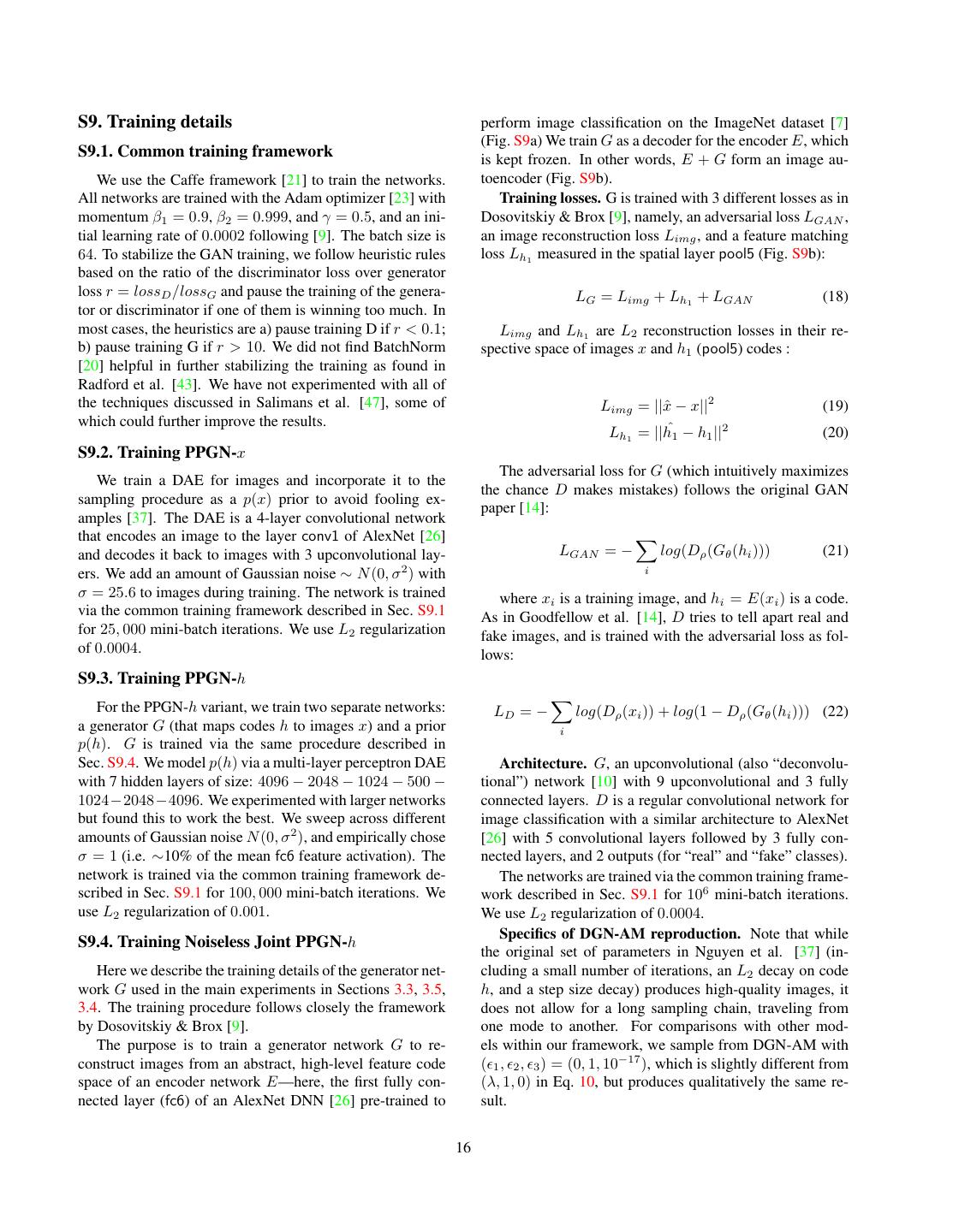
16 .S9. Training details perform image classification on the ImageNet dataset [7] (Fig. S9a) We train G as a decoder for the encoder E, which S9.1. Common training framework is kept frozen. In other words, E + G form an image au- We use the Caffe framework [21] to train the networks. toencoder (Fig. S9b). All networks are trained with the Adam optimizer [23] with Training losses. G is trained with 3 different losses as in momentum β1 = 0.9, β2 = 0.999, and γ = 0.5, and an ini- Dosovitskiy & Brox [9], namely, an adversarial loss LGAN , tial learning rate of 0.0002 following [9]. The batch size is an image reconstruction loss Limg , and a feature matching 64. To stabilize the GAN training, we follow heuristic rules loss Lh1 measured in the spatial layer pool5 (Fig. S9b): based on the ratio of the discriminator loss over generator loss r = lossD /lossG and pause the training of the genera- LG = Limg + Lh1 + LGAN (18) tor or discriminator if one of them is winning too much. In most cases, the heuristics are a) pause training D if r < 0.1; Limg and Lh1 are L2 reconstruction losses in their re- b) pause training G if r > 10. We did not find BatchNorm spective space of images x and h1 (pool5) codes : [20] helpful in further stabilizing the training as found in Radford et al. [43]. We have not experimented with all of the techniques discussed in Salimans et al. [47], some of x − x||2 Limg = ||ˆ (19) which could further improve the results. Lh = ||hˆ1 − h1 ||2 1 (20) S9.2. Training PPGN-x The adversarial loss for G (which intuitively maximizes We train a DAE for images and incorporate it to the the chance D makes mistakes) follows the original GAN sampling procedure as a p(x) prior to avoid fooling ex- paper [14]: amples [37]. The DAE is a 4-layer convolutional network that encodes an image to the layer conv1 of AlexNet [26] and decodes it back to images with 3 upconvolutional lay- LGAN = − log(Dρ (Gθ (hi ))) (21) ers. We add an amount of Gaussian noise ∼ N (0, σ 2 ) with i σ = 25.6 to images during training. The network is trained where xi is a training image, and hi = E(xi ) is a code. via the common training framework described in Sec. S9.1 As in Goodfellow et al. [14], D tries to tell apart real and for 25, 000 mini-batch iterations. We use L2 regularization fake images, and is trained with the adversarial loss as fol- of 0.0004. lows: S9.3. Training PPGN-h For the PPGN-h variant, we train two separate networks: LD = − log(Dρ (xi )) + log(1 − Dρ (Gθ (hi ))) (22) a generator G (that maps codes h to images x) and a prior i p(h). G is trained via the same procedure described in Sec. S9.4. We model p(h) via a multi-layer perceptron DAE Architecture. G, an upconvolutional (also “deconvolu- with 7 hidden layers of size: 4096 − 2048 − 1024 − 500 − tional”) network [10] with 9 upconvolutional and 3 fully 1024−2048−4096. We experimented with larger networks connected layers. D is a regular convolutional network for but found this to work the best. We sweep across different image classification with a similar architecture to AlexNet amounts of Gaussian noise N (0, σ 2 ), and empirically chose [26] with 5 convolutional layers followed by 3 fully con- σ = 1 (i.e. ∼10% of the mean fc6 feature activation). The nected layers, and 2 outputs (for “real” and “fake” classes). network is trained via the common training framework de- The networks are trained via the common training frame- scribed in Sec. S9.1 for 100, 000 mini-batch iterations. We work described in Sec. S9.1 for 106 mini-batch iterations. use L2 regularization of 0.001. We use L2 regularization of 0.0004. Specifics of DGN-AM reproduction. Note that while S9.4. Training Noiseless Joint PPGN-h the original set of parameters in Nguyen et al. [37] (in- Here we describe the training details of the generator net- cluding a small number of iterations, an L2 decay on code work G used in the main experiments in Sections 3.3, 3.5, h, and a step size decay) produces high-quality images, it 3.4. The training procedure follows closely the framework does not allow for a long sampling chain, traveling from by Dosovitskiy & Brox [9]. one mode to another. For comparisons with other mod- The purpose is to train a generator network G to re- els within our framework, we sample from DGN-AM with construct images from an abstract, high-level feature code ( 1 , 2 , 3 ) = (0, 1, 10−17 ), which is slightly different from space of an encoder network E—here, the first fully con- (λ, 1, 0) in Eq. 10, but produces qualitatively the same re- nected layer (fc6) of an AlexNet DNN [26] pre-trained to sult. 16 

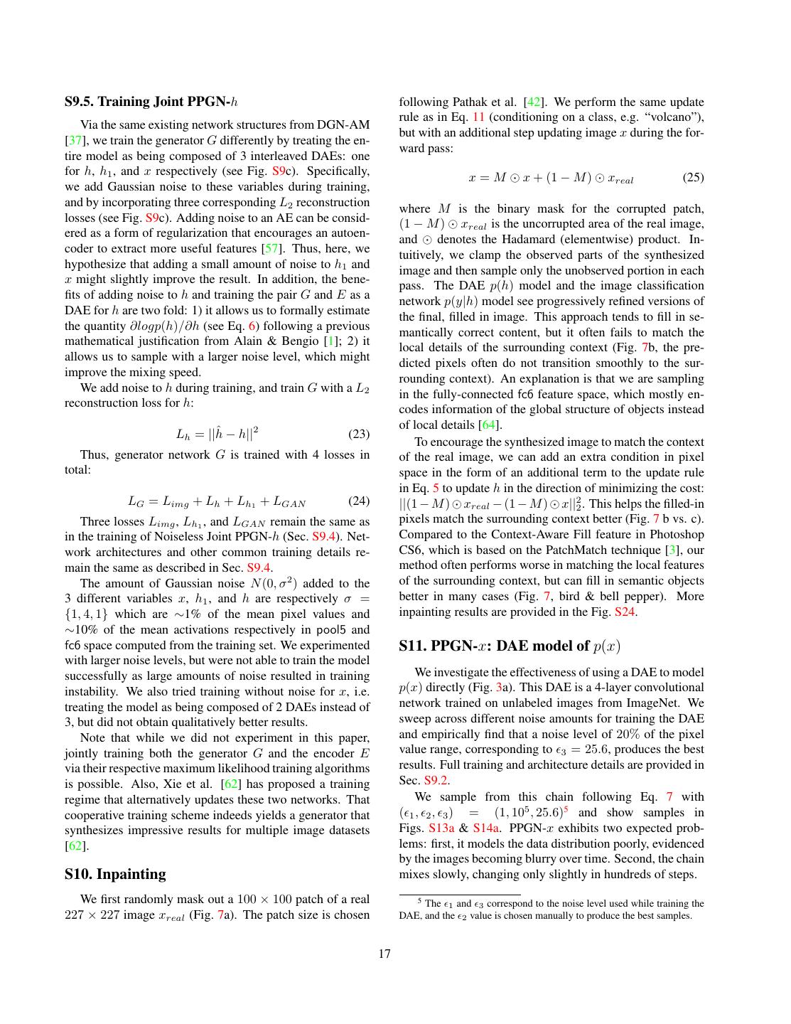
17 .S9.5. Training Joint PPGN-h following Pathak et al. [42]. We perform the same update rule as in Eq. 11 (conditioning on a class, e.g. “volcano”), Via the same existing network structures from DGN-AM but with an additional step updating image x during the for- [37], we train the generator G differently by treating the en- ward pass: tire model as being composed of 3 interleaved DAEs: one for h, h1 , and x respectively (see Fig. S9c). Specifically, x=M x + (1 − M ) xreal (25) we add Gaussian noise to these variables during training, and by incorporating three corresponding L2 reconstruction where M is the binary mask for the corrupted patch, losses (see Fig. S9c). Adding noise to an AE can be consid- (1 − M ) xreal is the uncorrupted area of the real image, ered as a form of regularization that encourages an autoen- and denotes the Hadamard (elementwise) product. In- coder to extract more useful features [57]. Thus, here, we tuitively, we clamp the observed parts of the synthesized hypothesize that adding a small amount of noise to h1 and image and then sample only the unobserved portion in each x might slightly improve the result. In addition, the bene- pass. The DAE p(h) model and the image classification fits of adding noise to h and training the pair G and E as a network p(y|h) model see progressively refined versions of DAE for h are two fold: 1) it allows us to formally estimate the final, filled in image. This approach tends to fill in se- the quantity ∂logp(h)/∂h (see Eq. 6) following a previous mantically correct content, but it often fails to match the mathematical justification from Alain & Bengio [1]; 2) it local details of the surrounding context (Fig. 7b, the pre- allows us to sample with a larger noise level, which might dicted pixels often do not transition smoothly to the sur- improve the mixing speed. rounding context). An explanation is that we are sampling We add noise to h during training, and train G with a L2 in the fully-connected fc6 feature space, which mostly en- reconstruction loss for h: codes information of the global structure of objects instead ˆ − h||2 of local details [64]. Lh = ||h (23) To encourage the synthesized image to match the context Thus, generator network G is trained with 4 losses in of the real image, we can add an extra condition in pixel total: space in the form of an additional term to the update rule in Eq. 5 to update h in the direction of minimizing the cost: LG = Limg + Lh + Lh1 + LGAN (24) ||(1 − M ) xreal − (1 − M ) x||22 . This helps the filled-in Three losses Limg , Lh1 , and LGAN remain the same as pixels match the surrounding context better (Fig. 7 b vs. c). in the training of Noiseless Joint PPGN-h (Sec. S9.4). Net- Compared to the Context-Aware Fill feature in Photoshop work architectures and other common training details re- CS6, which is based on the PatchMatch technique [3], our main the same as described in Sec. S9.4. method often performs worse in matching the local features The amount of Gaussian noise N (0, σ 2 ) added to the of the surrounding context, but can fill in semantic objects 3 different variables x, h1 , and h are respectively σ = better in many cases (Fig. 7, bird & bell pepper). More {1, 4, 1} which are ∼1% of the mean pixel values and inpainting results are provided in the Fig. S24. ∼10% of the mean activations respectively in pool5 and fc6 space computed from the training set. We experimented S11. PPGN-x: DAE model of p(x) with larger noise levels, but were not able to train the model successfully as large amounts of noise resulted in training We investigate the effectiveness of using a DAE to model instability. We also tried training without noise for x, i.e. p(x) directly (Fig. 3a). This DAE is a 4-layer convolutional treating the model as being composed of 2 DAEs instead of network trained on unlabeled images from ImageNet. We 3, but did not obtain qualitatively better results. sweep across different noise amounts for training the DAE Note that while we did not experiment in this paper, and empirically find that a noise level of 20% of the pixel jointly training both the generator G and the encoder E value range, corresponding to 3 = 25.6, produces the best via their respective maximum likelihood training algorithms results. Full training and architecture details are provided in is possible. Also, Xie et al. [62] has proposed a training Sec. S9.2. regime that alternatively updates these two networks. That We sample from this chain following Eq. 7 with cooperative training scheme indeeds yields a generator that ( 1 , 2 , 3 ) = (1, 105 , 25.6)5 and show samples in synthesizes impressive results for multiple image datasets Figs. S13a & S14a. PPGN-x exhibits two expected prob- [62]. lems: first, it models the data distribution poorly, evidenced by the images becoming blurry over time. Second, the chain S10. Inpainting mixes slowly, changing only slightly in hundreds of steps. We first randomly mask out a 100 × 100 patch of a real 5 The 1 and 3 correspond to the noise level used while training the 227 × 227 image xreal (Fig. 7a). The patch size is chosen DAE, and the 2 value is chosen manually to produce the best samples. 17 

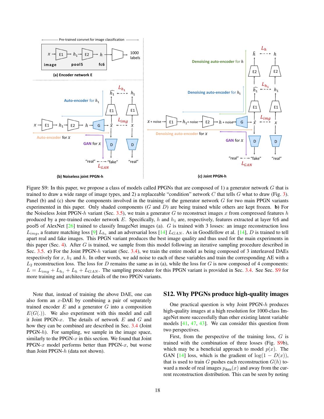
18 . Pre-­‐trained  convnet for  image  classification 𝐿- 𝑥 E1 ℎ$ E2 ℎ 1000 ℎ/ ℎ labels Denoising  auto-­‐encoder for  ℎ image pool5 fc6 E2 E2 B1 (a)  Encoder  network  E 𝐿-. 𝐿-. %$ ℎ ℎ$ %$ ℎ ℎ$ Denoising  auto-­‐encoder for  ℎ$ Auto-­‐encoder for  ℎ$ E1 E1 B1 E1 E1 B1 𝐿'() 𝐿'() 𝑥 +  noise E1 ℎ$+  noise E2 ℎ +  noise G 𝑥" 𝑥 𝑥 E1 ℎ$ E2 ℎ G 𝑥" 𝑥 Denoising  auto-­‐encoder for 𝑥 Auto-­‐encoder for 𝑥 GAN for 𝑥 D D GAN for 𝑥 D D “real” “fake” “real” “real” “fake” “real” 𝐿*+, 𝐿*+, (b)  Noiseless  joint  PPGN-­‐h (c)  Joint  PPGN-­‐h Figure S9: In this paper, we propose a class of models called PPGNs that are composed of 1) a generator network G that is trained to draw a wide range of image types, and 2) a replaceable “condition” network C that tells G what to draw (Fig. 3). Panel (b) and (c) show the components involved in the training of the generator network G for two main PPGN variants experimented in this paper. Only shaded components (G and D) are being trained while others are kept frozen. b) For the Noiseless Joint PPGN-h variant (Sec. 3.5), we train a generator G to reconstruct images x from compressed features h produced by a pre-trained encoder network E. Specifically, h and h1 are, respectively, features extracted at layer fc6 and pool5 of AlexNet [26] trained to classify ImageNet images (a). G is trained with 3 losses: an image reconstruction loss Limg , a feature matching loss [9] Lh1 and an adversarial loss [14] LGAN . As in Goodfellow et al. [14], D is trained to tell apart real and fake images. This PPGN variant produces the best image quality and thus used for the main experiments in this paper (Sec. 4). After G is trained, we sample from this model following an iterative sampling procedure described in Sec. 3.5. c) For the Joint PPGN-h variant (Sec. 3.4), we train the entire model as being composed of 3 interleaved DAEs respectively for x, h1 and h. In other words, we add noise to each of these variables and train the corresponding AE with a L2 reconstruction loss. The loss for D remains the same as in (a), while the loss for G is now composed of 4 components: L = Limg + Lh1 + Lh + LGAN . The sampling procedure for this PPGN variant is provided in Sec. 3.4. See Sec. S9 for more training and architecture details of the two PPGN variants. Note that, instead of training the above DAE, one can S12. Why PPGNs produce high-quality images also form an x-DAE by combining a pair of separately trained encoder E and a generator G into a composition One practical question is why Joint PPGN-h produces E(G(.)). We also experiment with this model and call high-quality images at a high resolution for 1000-class Im- it Joint PPGN-x. The details of network E and G and ageNet more successfully than other existing latent variable how they can be combined are described in Sec. 3.4 (Joint models [41, 47, 43]. We can consider this question from PPGN-h). For sampling, we sample in the image space, two perspectives. similarly to the PPGN-x in this section. We found that Joint First, from the perspective of the training loss, G is PPGN-x model performs better than PPGN-x, but worse trained with the combination of three losses (Fig. S9b), than Joint PPGN-h (data not shown). which may be a beneficial approach to model p(x). The GAN [14] loss, which is the gradient of log(1 − D(x)), that is used to train G pushes each reconstruction G(h) to- ward a mode of real images pdata (x) and away from the cur- rent reconstruction distribution. This can be seen by noting 18 

19 .that the Bayes optimal D is pdata (x)/(pdata (x) + pmodel (x)) [14]. Since x ∼ G(h) is already near a mode of pmodel (x), the net effect is to push G(h) towards one of the modes of pdata , thus making the reconstructions sharper and more plausible. If one uses only the GAN objective and no re- construction objectives (L2 losses in the pixel or feature space), G may bring the sample far from the original x, pos- sibly collapsing several modes of x into fewer modes. This is the typical, known “missing-mode” behavior of GANs [47, 14] that arises in part because GANs minimize the Jensen-Shannon divergence rather than Kullback-Leibler divergence between pdata and pmodel , leading to an over- memorization of modes [53]. The reconstruction losses are important to combat this missing mode problem and may also serve to enable better convergence of the feature space autoencoder to the distribution it models, which is neces- sary in order to make the h-space reconstruction properly estimate ∂ log p(h)/∂h [1]. Second, from the perspective of the learned h → x map- ping, we train the G parameters of the E + G pair of net- works as an x-AE, mapping x → h → x (see Fig. S9b). In this configuration, as in VAEs [24] and regular DAEs [57], the one-to-one mapping helps prevent the typical la- tent → input missing mode collapse that occurs in GANs, where some input images are not representable using any code [14, 47]. However, unlike in VAEs and DAEs, where the latent distribution is learned in a purely unsupervised manner, we leverage the labeled ImageNet data to train E in a supervised manner that yields a distribution of features h that we hypothesize to be semantically meaningful and useful for building a generative image model. To further understand the effectiveness of using deep, supervised fea- tures, it might be interesting future work to train PPGNs with other feature distributions h such as random features or shallow features (e.g. produced by PCA). 19 

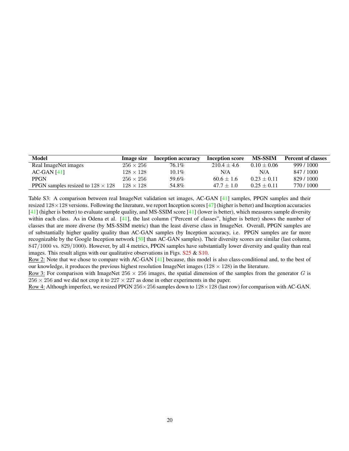
20 . Model Image size Inception accuracy Inception score MS-SSIM Percent of classes Real ImageNet images 256 × 256 76.1% 210.4 ± 4.6 0.10 ± 0.06 999 / 1000 AC-GAN [41] 128 × 128 10.1% N/A N/A 847 / 1000 PPGN 256 × 256 59.6% 60.6 ± 1.6 0.23 ± 0.11 829 / 1000 PPGN samples resized to 128 × 128 128 × 128 54.8% 47.7 ± 1.0 0.25 ± 0.11 770 / 1000 Table S3: A comparison between real ImageNet validation set images, AC-GAN [41] samples, PPGN samples and their resized 128×128 versions. Following the literature, we report Inception scores [47] (higher is better) and Inception accuracies [41] (higher is better) to evaluate sample quality, and MS-SSIM score [41] (lower is better), which measures sample diversity within each class. As in Odena et al. [41], the last column (“Percent of classes”, higher is better) shows the number of classes that are more diverse (by MS-SSIM metric) than the least diverse class in ImageNet. Overall, PPGN samples are of substantially higher quality quality than AC-GAN samples (by Inception accuracy, i.e. PPGN samples are far more recognizable by the Google Inception network [50] than AC-GAN samples). Their diversity scores are similar (last column, 847/1000 vs. 829/1000). However, by all 4 metrics, PPGN samples have substantially lower diversity and quality than real images. This result aligns with our qualitative observations in Figs. S25 & S10. Row 2: Note that we chose to compare with AC-GAN [41] because, this model is also class-conditional and, to the best of our knowledge, it produces the previous highest resolution ImageNet images (128 × 128) in the literature. Row 3: For comparison with ImageNet 256 × 256 images, the spatial dimension of the samples from the generator G is 256 × 256 and we did not crop it to 227 × 227 as done in other experiments in the paper. Row 4: Although imperfect, we resized PPGN 256×256 samples down to 128×128 (last row) for comparison with AC-GAN. 20 

21 . (a) Real: top 9 (b) DGN-AM [37] (c) Real: random 9 (d) PPGN (this) Figure S10: (a) The 9 training set images that most highly activate a given class output neuron (e.g. fire engine). (b) DGN- AM [37] synthesizes high-quality images, but they often converge to the mode of high-activating images (the top-9 mode). (c) 9 training set images randomly picked from the same class. (d) Our new method PPGN produces samples with better quality and substantially larger diversity than DGN-AM, thus better representing the diversity of images from the class. 21 

22 . (a) Samples produced by PPGN visualized in a grid t-SNE [56] . (b) Samples hand-picked from (a) to showcase the diversity and quality of images produced by PPGN. Figure S11: We qualitatively evaluate sample diversity by running 10 sampling chains (conditioned on class “volcano”), each for 200 steps, to produce 2000 samples, and filtering out samples with class probability of less than 0.97. From the remaining, we randomly pick 400 samples and plot them in a grid t-SNE [56] (top panel). From those, we chose a selection to highlight the quality and diversity of the samples (bottom panel). There is a tremendous amount of detail in each image and diversity across images. Samples include dormant volcanos and active22 volcanoes with smoke plumes of different colors from white to black to fiery orange. Some have two peaks and others one, and underneath are scree, green forests, or glaciers (complete with crevasses). The sky changes from different shades of mid-day blue through different sunsets to pitch black night. 

23 . (a) Samples produced by PPGN visualized in a grid t-SNE [56] . (b) Samples hand-picked from (a) to showcase the diversity and quality of images produced by PPGN. Figure S12: The figures are selected and plotted in the same way as Fig. S11, but here for the “pool table” class. Once again, we observe a high degree of both image quality and diversity. Different felt colors (green, blue, and red), lighting conditions, camera angles, and interior designs are apparent. 23 

24 . (a) PPGN-x with a DAE model of p(x) (b) DGN-AM [37] (which has a hand-designed Gaussian p(h) prior) (c) PPGN-h: Generator and multi-layer perceptron DAE model of p(h) (d) Joint PPGN-h: joint Generator and DAE (e) Noiseless Joint PPGN-h: joint Generator and AE Figure S13: A comparison of samples generated from a single sampling chain (starting from a real image on the left) across different models. Each panel shows two sampling chains for that model: one conditioned on the “planetarium” class and the other conditioned on the “kite” (a type of bird) class. The iteration number of the sampling chain is shown on top. (a) The sampling chain in the image space mixes poorly. (b) The sampling chain from DGN-AM [37] (in the h code space with a hand-designed Gaussian p(h) prior) produces better images, but still mixes poorly, as evidenced by similar samples over many iterations. (c) To improve sampling, we tried swapping in a p(h) model represented by a 7-layer DAE for h. However, the sampling chain does not mix faster or produce better samples. (d) We experimented with a better way to model p(h), i.e. modeling h via x. We treat the generator G and encoder E as an autoencoder for h and call this treatment “Noiseless Joint PPGN-h” (see Sec. 3.5). This is also our best model that we use for experiments in Sec. 4. This substantially improves the mixing speed and sample quality. (e) We train the entire model 24 as being composed of 3 DAEs and sample from it by adding noise to the image, fc6 and pool5 variables. The chain mixes slightly faster compared to (d), but generates slightly worse samples. 

25 . (a) PPGN-x with a DAE model of p(x) (b) DGN-AM [37] (which has a hand-designed Gaussian p(h) prior) (c) PPGN-h: Generator and a multi-layer perceptron DAE model of p(h) (d) Joint PPGN-h: joint Generator and DAE (e) Noiseless Joint PPGN-h: joint Generator and AE Figure S14: Same as Fig. S13, but starting from a random code h (which when pushed through generator network G produces the leftmost images) except for (a) which starts from random images as the sampling operates directly in the pixel space. All of our qualitative conclusions are the same as for Fig. S13. Note that the samples in (b) appear slightly worse than the images reported in Nguyen et al. [37]. The reason is that in the new framework introduced in this paper we perform an infinitely long sampling chain at a constant learning rate to travel from one mode to another in the space. In contrast, the set of parameters (including the number of iterations, an L2 decay on code h, and a learning rate decay) in Nguyen et al. [37] is carefully tuned for the best image quality, but does not allow for a long sampling chain (Fig. 2). 25 

26 . (a) Very large noise ( 3 = 10−1 ) (b) Large noise ( 3 = 10−5 ) (c) Medium noise ( 3 = 10−9 ) (d) Small noise ( 3 = 10−13 ) (e) Infinitesimal noise ( 3 = 10−17 ) Figure S15: Sampling chains with the noiseless PPGN model starting from the code of a real image (left) and conditioning on class “planetarium” i.e. ( 1 , 2 ) = (1, 10−5 ) for different noise levels 3 . The sampling step numbers are shown on top. Samples are better with a tiny amount of noise (e) than with larger noise levels (a,b,c & d), so we chose that as our default noise level for all sampling experiments with the Noiseless Joint PPGN-h variant (Sec. 3.5). These results suggest that a certain amount of noise added to the DAE during training might help the chain mix faster, and thus partly motivated our experiment in Sec. 3.4. 26 

27 .Figure S16: The default generator network G in our experiments (used in Sections 3.3 & 3.5) was trained to reconstruct im- ages from compressed fc6 features extracted from AlexNet classification network [26] with three different losses: adversarial loss [14], feature matching loss [9], and image reconstruction loss (more training details are in Sec. S9.4). Here, we test how robust G is to Gaussian noise added to an input code h of a real image. We sweep across different levels of Gaussian noise N (0, σ 2 ) with σ = {1%, 10%, 20%, 30%, 40%} of the mean fc6 activation computed by the activations of validation set images. We observed that G is robust to even a large amount of noise up to σ = 20% despite being trained without explicit regularizations (i.e. with noise [57] or a contractive penalty [44]). 27 

28 . (a) Samples produced by the DGN-AM method [37] (b) Samples produced by PPGN (the new model proposed in this paper) Figure S17: A comparison of images produced by the DGN-AM method [37] (top) and the new PPGN method we introduce in this paper (bottom). Both methods synthesize images conditioned on classes of scene images that the generator was never trained on. Specifically, the condition model p(y|x) is AlexNet trained to classify 205 categories of scene images from the MIT Places dataset [65], while the prior model p(x) is trained to generate ImageNet images. Despite having a strong, learned prior (represented by a DAE trained on ImageNet images), the PPGN (like DGN-AM) produces high-quality images for an unseen dataset. 28 

29 .Figure S18: The model can be given a text description of an image and asked to generate the described image. Technically, that involves the same PPGN model, but conditioning on a caption instead of a class. Here the condition network is the LRCN image captioning model from Donahue et al. [8], which can generate reasonable captions for images. For each caption, we show 4 images synthesized by starting from random initializations. Note that it reasonably draws “tarmac”, “silhouette” or “woman” although these are not categories in the ImageNet dataset [7]. 29