10-Pipeline Pattern

1 . Pipeline Pattern Parallel Computing CIS 410/510 Department of Computer and Information Science Lecture 10 – Pipeline 

2 . Outline q  What is the pipeline concept? q  What is the pipeline pattern? q  Example: Bzip2 data compression q  Implementation strategies q  Pipelines in TBB q  Pipelines in Cilk Plus q  Example: parallel Bzip2 data compression q  Mandatory parallelism vs. optional parallelism Introduction to Parallel Computing, University of Oregon, IPCC Lecture 10 – Pipeline 2 

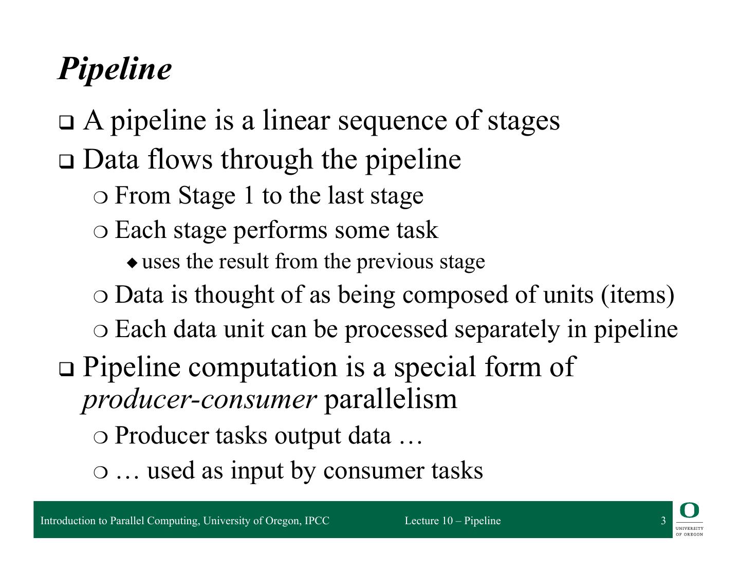
3 . Pipeline q  Apipeline is a linear sequence of stages q  Data flows through the pipeline ❍  From Stage 1 to the last stage ❍  Each stage performs some task ◆ uses the result from the previous stage ❍  Data is thought of as being composed of units (items) ❍  Each data unit can be processed separately in pipeline q  Pipeline computation is a special form of producer-consumer parallelism ❍  Producertasks output data … ❍  … used as input by consumer tasks Introduction to Parallel Computing, University of Oregon, IPCC Lecture 10 – Pipeline 3 

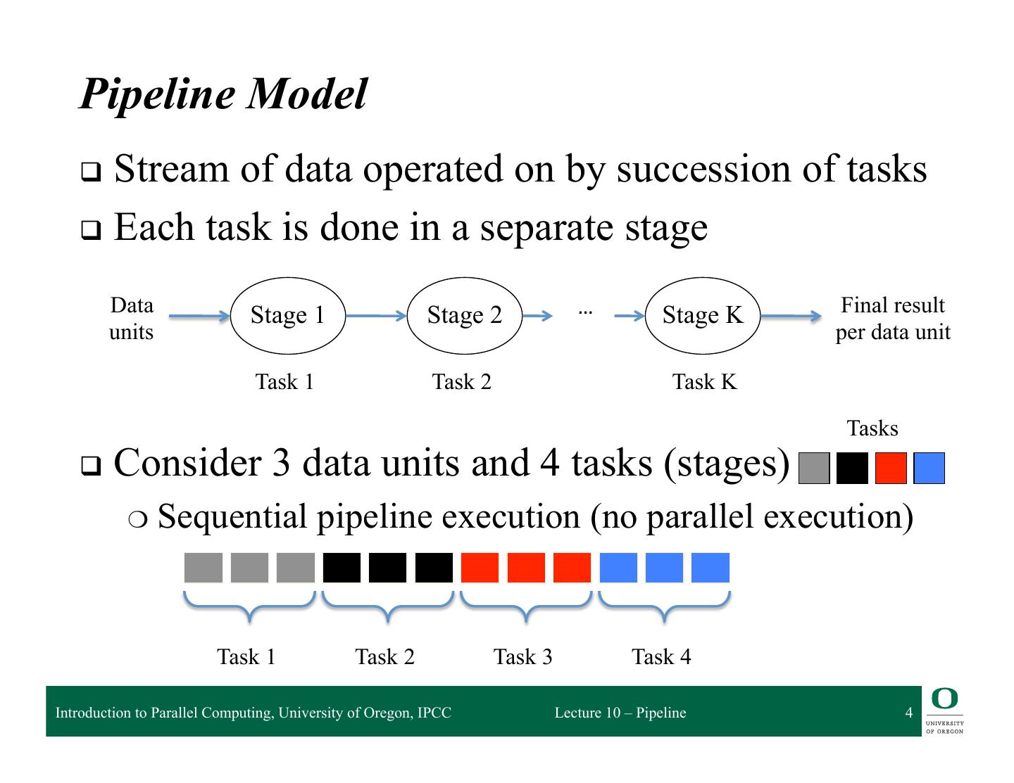
4 . Pipeline Model q  Stream of data operated on by succession of tasks q  Each task is done in a separate stage Data Stage 1 Stage 2 …   Stage K Final result units per data unit Task 1 Task 2 Task K Tasks q  Consider 3 data units and 4 tasks (stages) ❍  Sequential pipeline execution (no parallel execution) Task 1 Task 2 Task 3 Task 4 Introduction to Parallel Computing, University of Oregon, IPCC Lecture 10 – Pipeline 4 

5 . Where is the Concurrency? (Serial Pipeline) q  Pipeline with serial stages ❍  Each stage runs serially (i.e., can not be parallel) ❍  Can not parallelize the tasks q  What can we run in parallel? ❍  Think about data parallelism ❍  Provide a separate pipeline for each data item Processor 1 2 3 4 3 data items 5 data items 5 q  What do you notice as we increase # data items? Introduction to Parallel Computing, University of Oregon, IPCC Lecture 10 – Pipeline 5 

6 . Parallelizing Serial Pipelines q  # tasks limits the parallelism with serial tasks Processor 1 2 3 4 3 data items 5 data items 5 q  Two parallel execution choices: 1) processor executes the entire pipeline 2) processor assigned to execute a single task q  Which is better? Why? Introduction to Parallel Computing, University of Oregon, IPCC Lecture 10 – Pipeline 6 

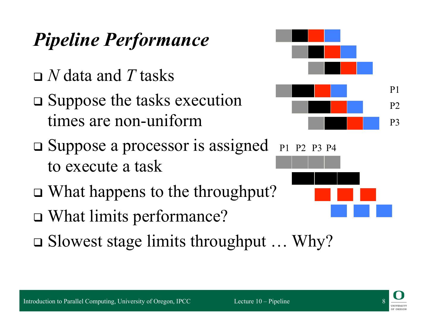
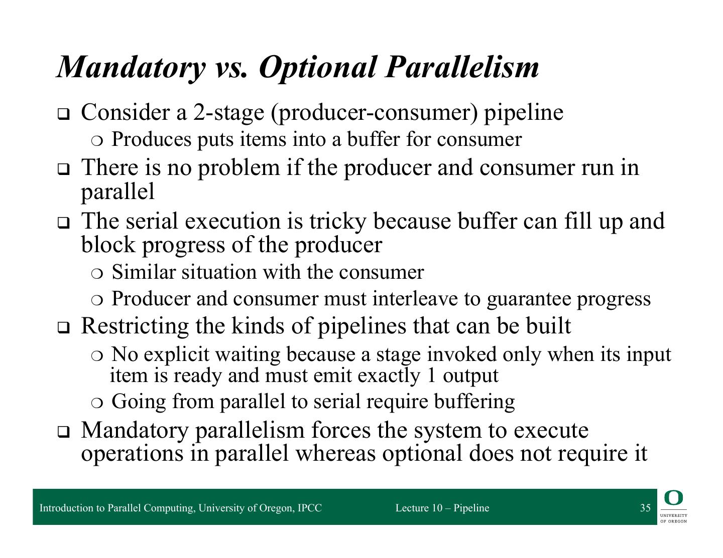
7 . Pipeline Performance q  N data and T tasks q  Each task takes unit time t q  Sequential time = N*T*t q  Parallel pipeline time = start + finish + (N-2T)/T * t = O(N/T) (for N>>T) q  Try to find a lot of data to pipeline q  Try to divide computation in a lot of pipeline tasks ❍  More tasks to do (longer pipelines) ❍  Break a larger task into more (shorter) tasks to do q  Interested in pipeline throughput Introduction to Parallel Computing, University of Oregon, IPCC Lecture 10 – Pipeline 7 

8 . Pipeline Performance q  N data and T tasks P1 q  Suppose the tasks execution P2 times are non-uniform P3 q  Suppose a processor is assigned P1 P2 P3 P4 to execute a task q  What happens to the throughput? q  What limits performance? q  Slowest stage limits throughput … Why? Introduction to Parallel Computing, University of Oregon, IPCC Lecture 10 – Pipeline 8 

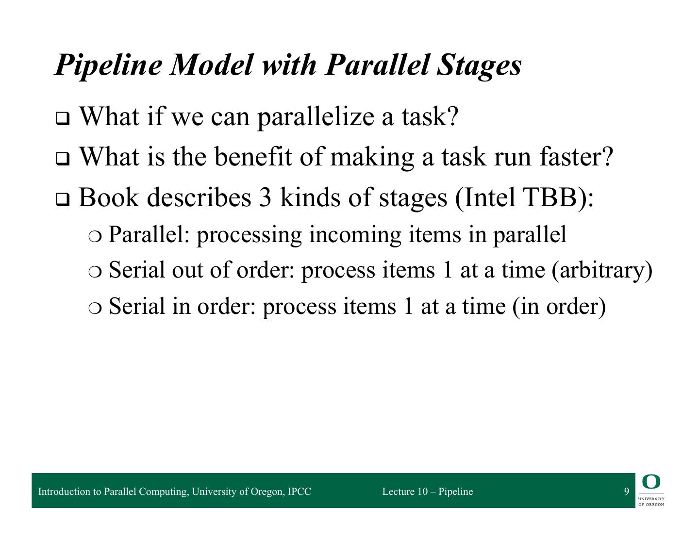
9 . Pipeline Model with Parallel Stages q  What if we can parallelize a task? q  What is the benefit of making a task run faster? q  Book describes 3 kinds of stages (Intel TBB): ❍  Parallel: processing incoming items in parallel ❍  Serial out of order: process items 1 at a time (arbitrary) ❍  Serial in order: process items 1 at a time (in order) Introduction to Parallel Computing, University of Oregon, IPCC Lecture 10 – Pipeline 9 

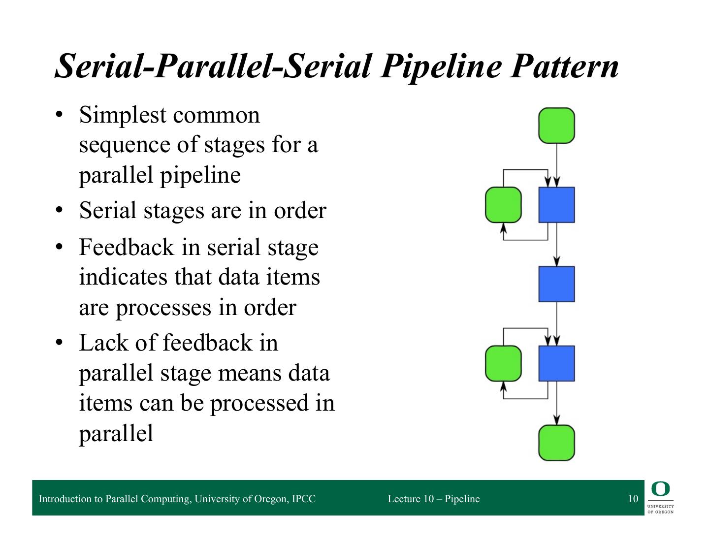
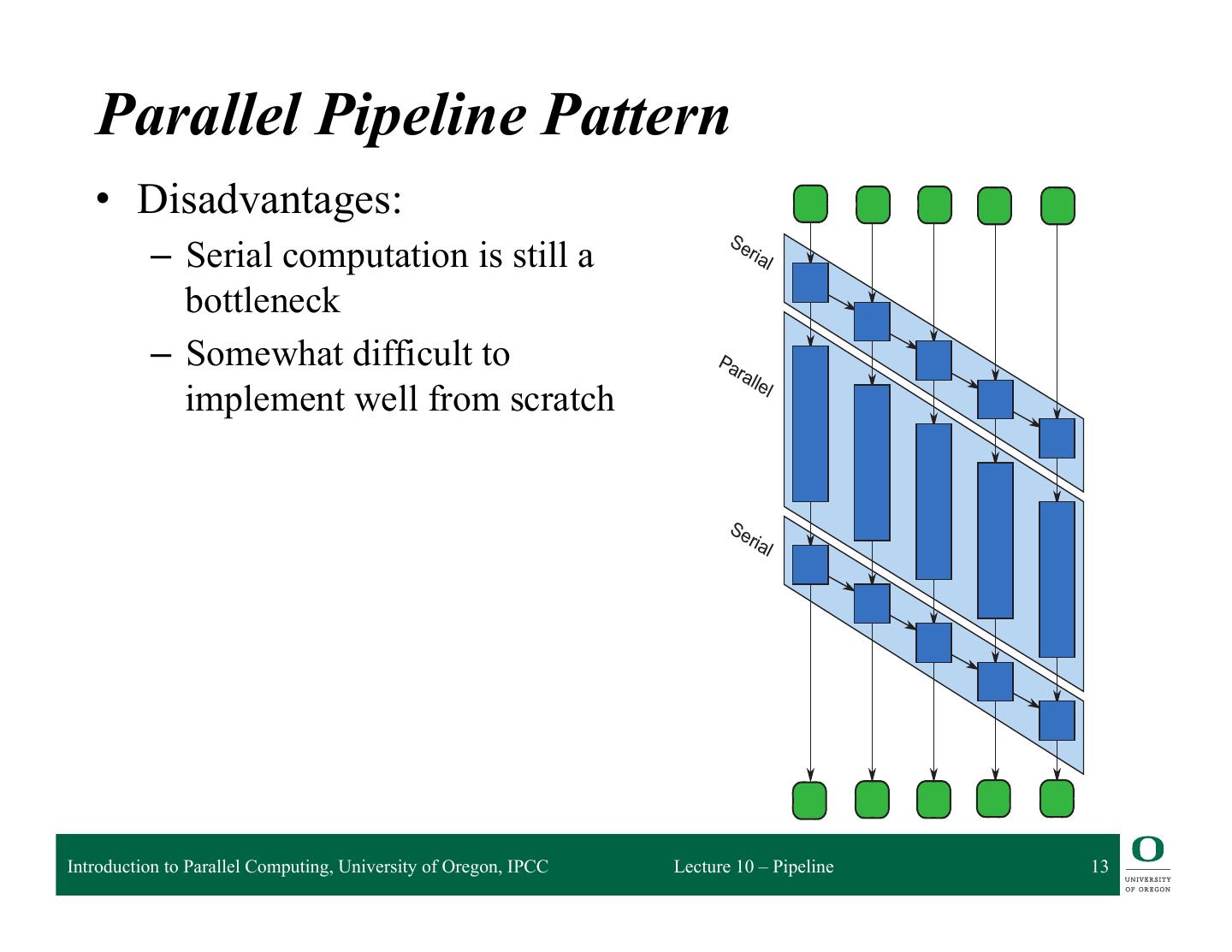
10 . Serial-Parallel-Serial Pipeline Pattern •  Simplest common sequence of stages for a parallel pipeline •  Serial stages are in order •  Feedback in serial stage indicates that data items are processes in order •  Lack of feedback in parallel stage means data items can be processed in parallel Introduction to Parallel Computing, University of Oregon, IPCC Lecture 10 – Pipeline 10 

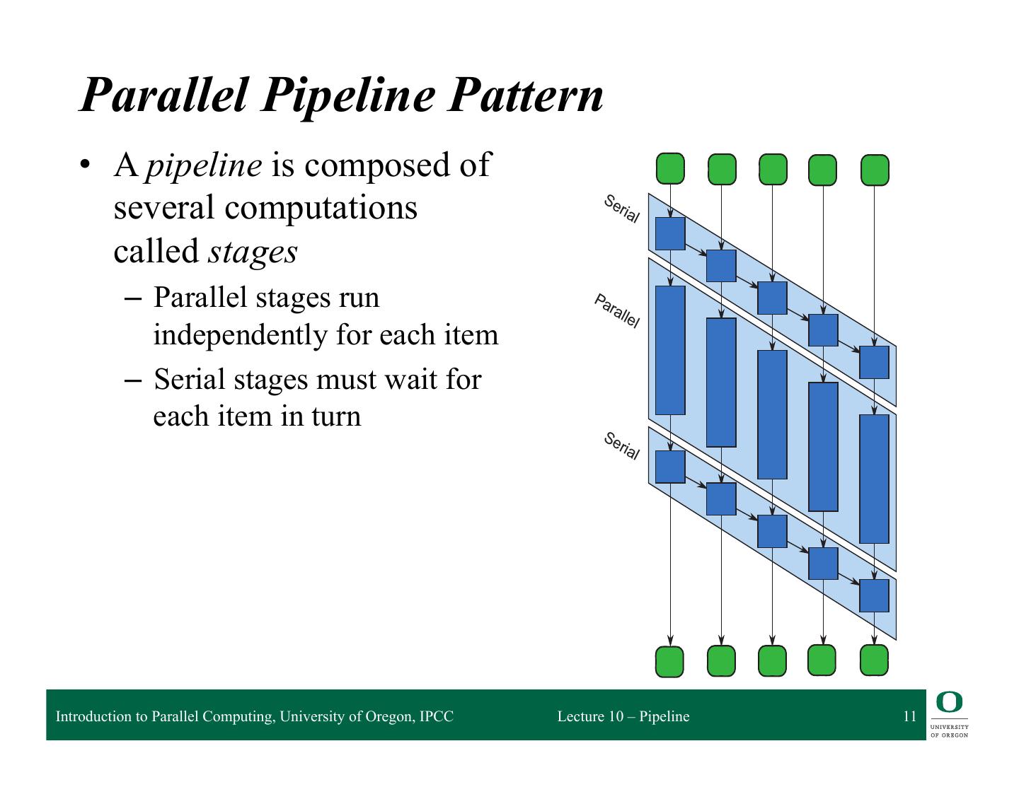
11 . it up when the stage is ready to accept it. After a worker finishes applying a serial stage checks if there is a parked input item waiting at that state, and if so spawns a task that item and continues carrying it through the pipeline. In this way, execution of a serial stage without a mutex. Parallel Pipeline Pattern •  A pipeline is composed of several computations Se ria l called stages –  Parallel stages run Pa ral lel independently for each item –  Serial stages must wait for each item in turn Se ria l FIGURE IPCC Introduction to Parallel Computing, University of Oregon, 9.2 Lecture 10 – Pipeline 11 DAG model of pipeline in Figure 9.1. This picture shows the DAG model of computation (Section the pipeline in Figure 9.1, assuming there are five input items. To emphasize the opportunity for 

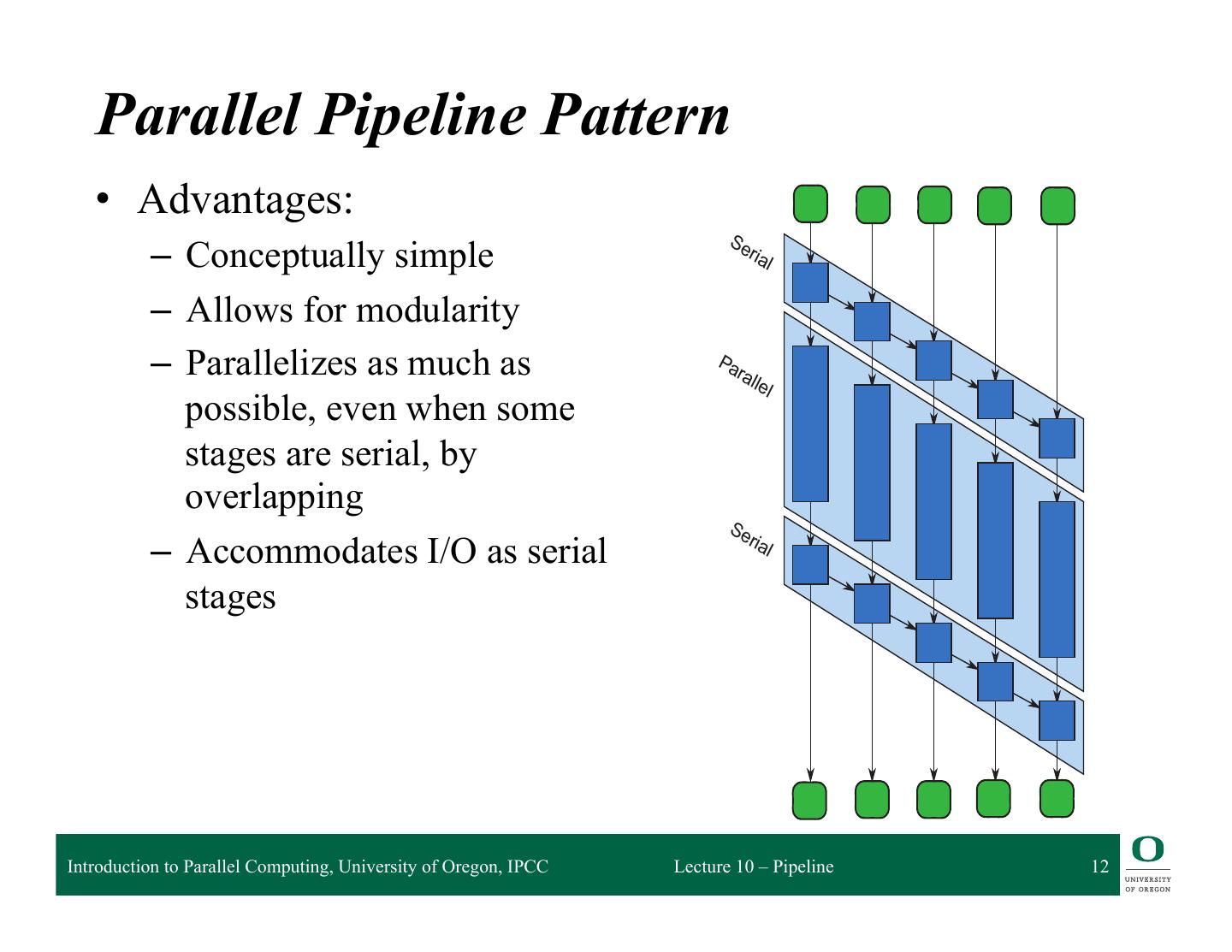
12 . it up when the stage is ready to accept it. After a worker finishes applying a serial stage checks if there is a parked input item waiting at that state, and if so spawns a task that item and continues carrying it through the pipeline. In this way, execution of a serial stage without a mutex. Parallel Pipeline Pattern •  Advantages: Se –  Conceptually simple ria l –  Allows for modularity –  Parallelizes as much as Pa ral lel possible, even when some stages are serial, by overlapping Se ria –  Accommodates I/O as serial l stages FIGURE IPCC Introduction to Parallel Computing, University of Oregon, 9.2 Lecture 10 – Pipeline 12 DAG model of pipeline in Figure 9.1. This picture shows the DAG model of computation (Section the pipeline in Figure 9.1, assuming there are five input items. To emphasize the opportunity for 

13 . it up when the stage is ready to accept it. After a worker finishes applying a serial stage checks if there is a parked input item waiting at that state, and if so spawns a task that item and continues carrying it through the pipeline. In this way, execution of a serial stage without a mutex. Parallel Pipeline Pattern •  Disadvantages: Se –  Serial computation is still a ria l bottleneck –  Somewhat difficult to Pa ral le implement well from scratch l Se ria l FIGURE IPCC Introduction to Parallel Computing, University of Oregon, 9.2 Lecture 10 – Pipeline 13 DAG model of pipeline in Figure 9.1. This picture shows the DAG model of computation (Section the pipeline in Figure 9.1, assuming there are five input items. To emphasize the opportunity for 

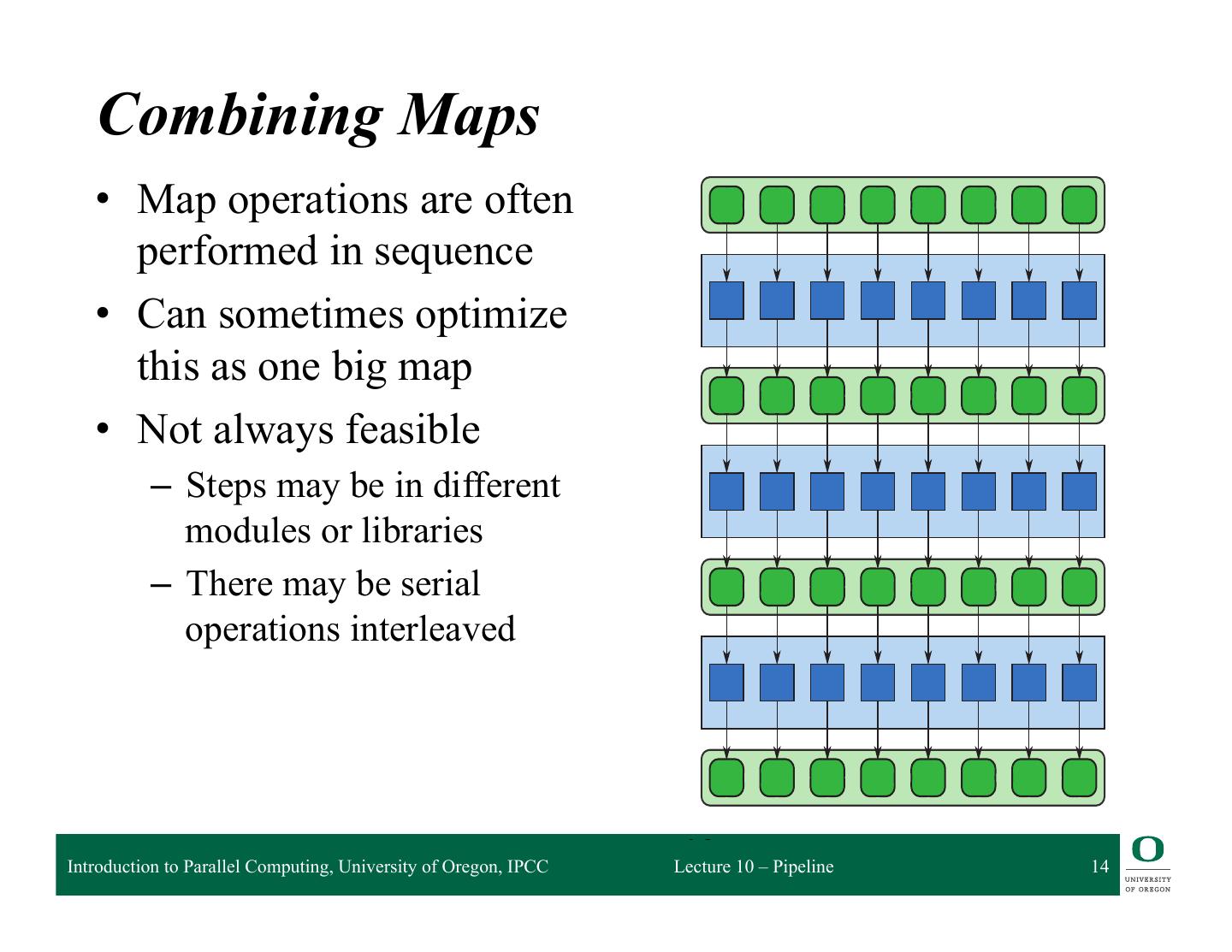
14 . If we fuse the operations used in a sequence of maps into load only the input data at the start of the map and keep int wasting memory bandwidth on them. We will call this appro other patterns as well. Code fusion is demonstrated in Figure Combining Maps •  Map operations are often performed in sequence •  Can sometimes optimize this as one big map •  Not always feasible –  Steps may be in different modules or libraries –  There may be serial operations interleaved FIGURE 4.2 Introduction to Parallel Computing, University of Oregon, IPCC Lecture 10 – Pipeline 14 Code fusion optimization: Convert a sequence of maps into a map intermediate results to memory. This can be done automatically by 

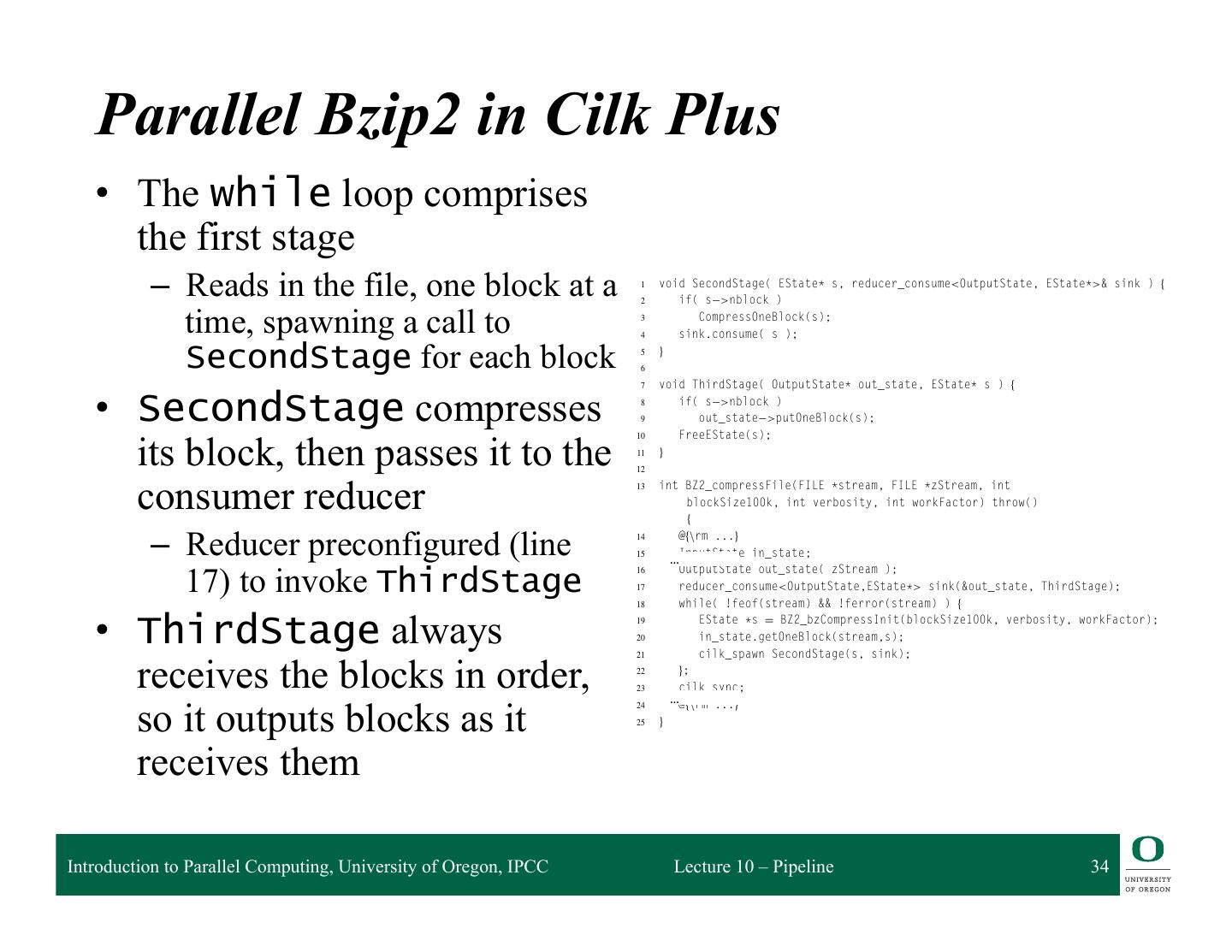
15 . Example: Bzip2 Data Compression q  bzip2 utility provides general-purpose data compression ❍  Better compression than gzip, but slower q  The algorithm operates in blocks ❍  Blocksare compressed independently ❍  Some pre- and post-processing must be done serially Introduction to Parallel Computing, University of Oregon, IPCC Lecture 10 – Pipeline 15 

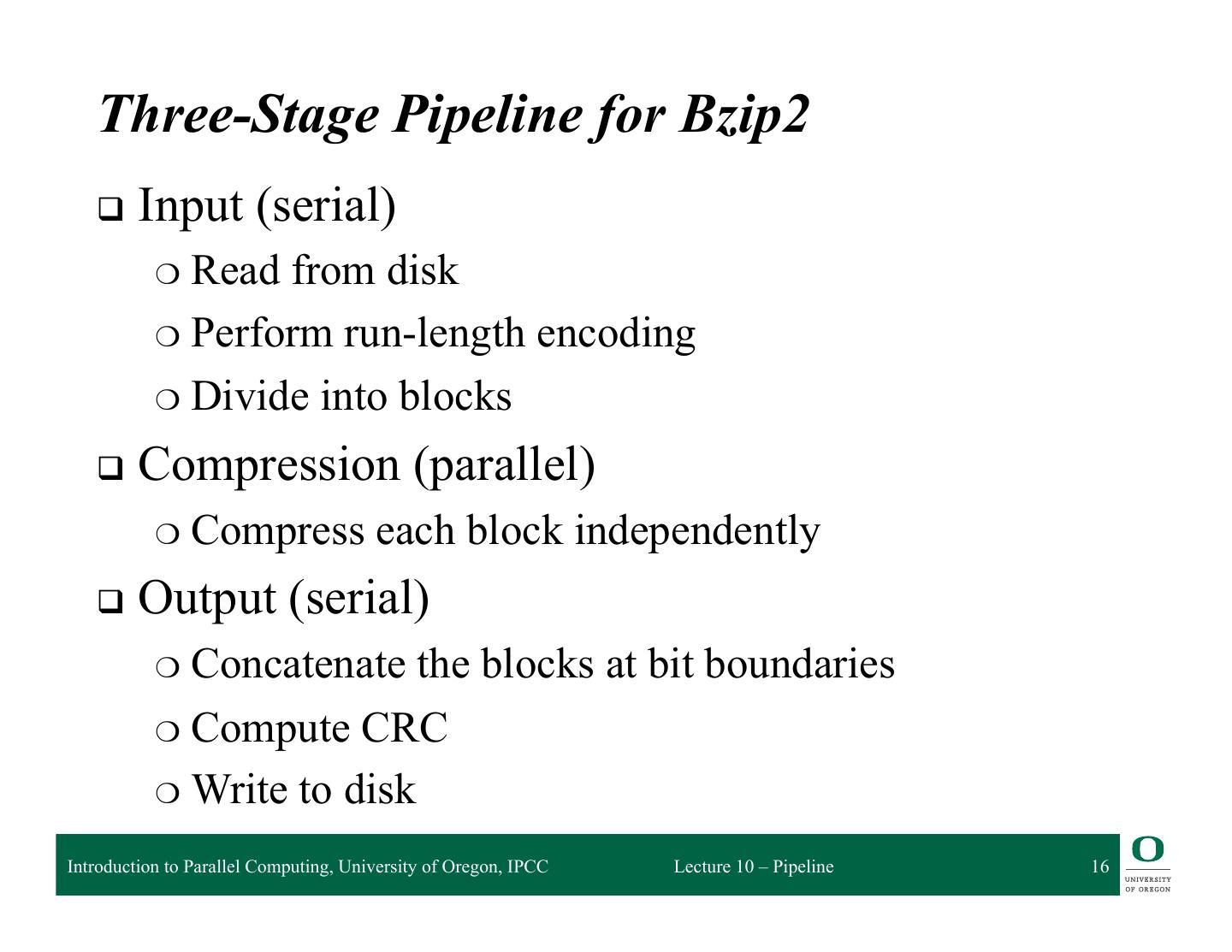
16 . Three-Stage Pipeline for Bzip2 q  Input (serial) ❍  Read from disk ❍  Perform run-length encoding ❍  Divide into blocks q  Compression (parallel) ❍  Compress each block independently q  Output (serial) ❍  Concatenate the blocks at bit boundaries ❍  Compute CRC ❍  Write to disk Introduction to Parallel Computing, University of Oregon, IPCC Lecture 10 – Pipeline 16 

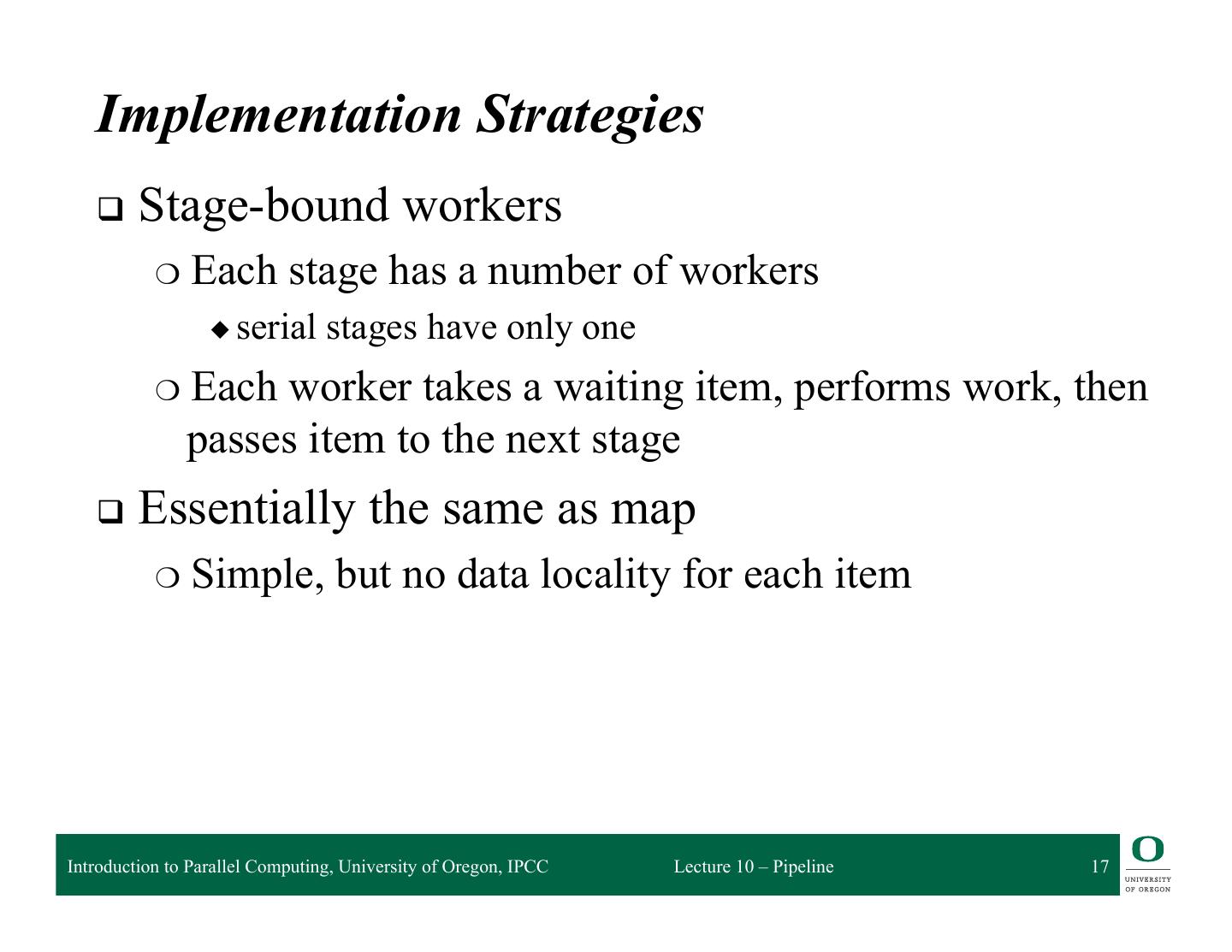
17 . Implementation Strategies q  Stage-bound workers ❍  Each stage has a number of workers ◆ serial stages have only one ❍  Each worker takes a waiting item, performs work, then passes item to the next stage q  Essentially the same as map ❍  Simple, but no data locality for each item Introduction to Parallel Computing, University of Oregon, IPCC Lecture 10 – Pipeline 17 

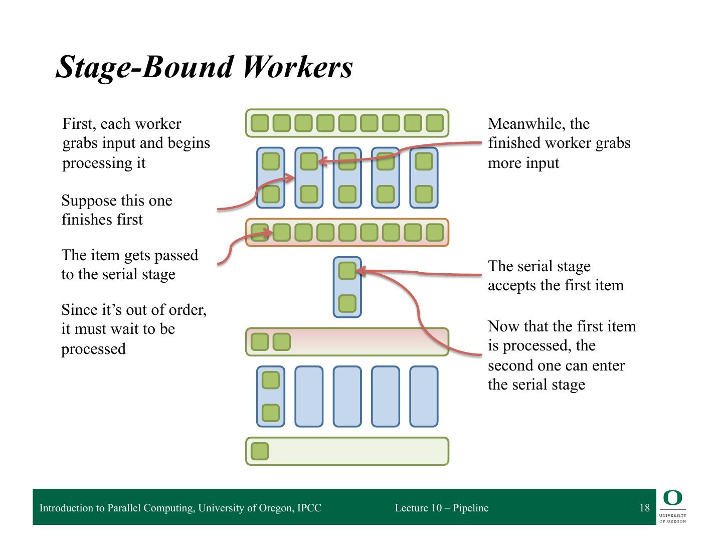
18 . Stage-Bound Workers First, each worker Meanwhile, the grabs input and begins finished worker grabs processing it more input Suppose this one finishes first The item gets passed The serial stage to the serial stage accepts the first item Since it’s out of order, it must wait to be Now that the first item processed is processed, the second one can enter the serial stage Introduction to Parallel Computing, University of Oregon, IPCC Lecture 10 – Pipeline 18 

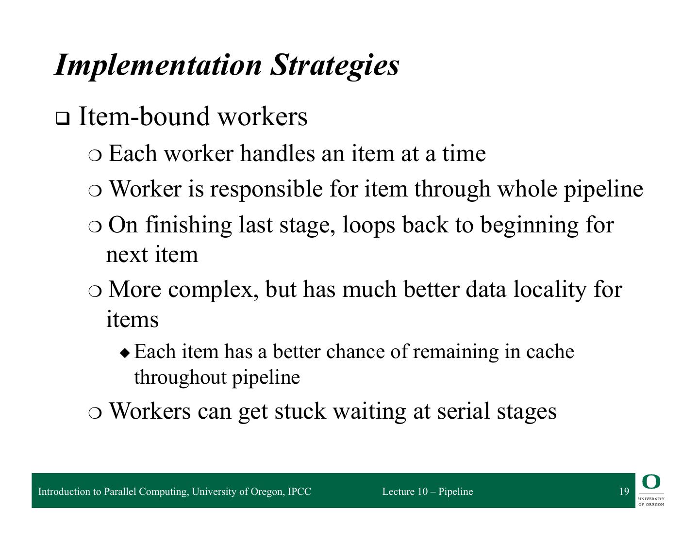
19 . Implementation Strategies q  Item-bound workers ❍  Each worker handles an item at a time ❍  Worker is responsible for item through whole pipeline ❍  On finishing last stage, loops back to beginning for next item ❍  More complex, but has much better data locality for items ◆ Each item has a better chance of remaining in cache throughout pipeline ❍  Workers can get stuck waiting at serial stages Introduction to Parallel Computing, University of Oregon, IPCC Lecture 10 – Pipeline 19 

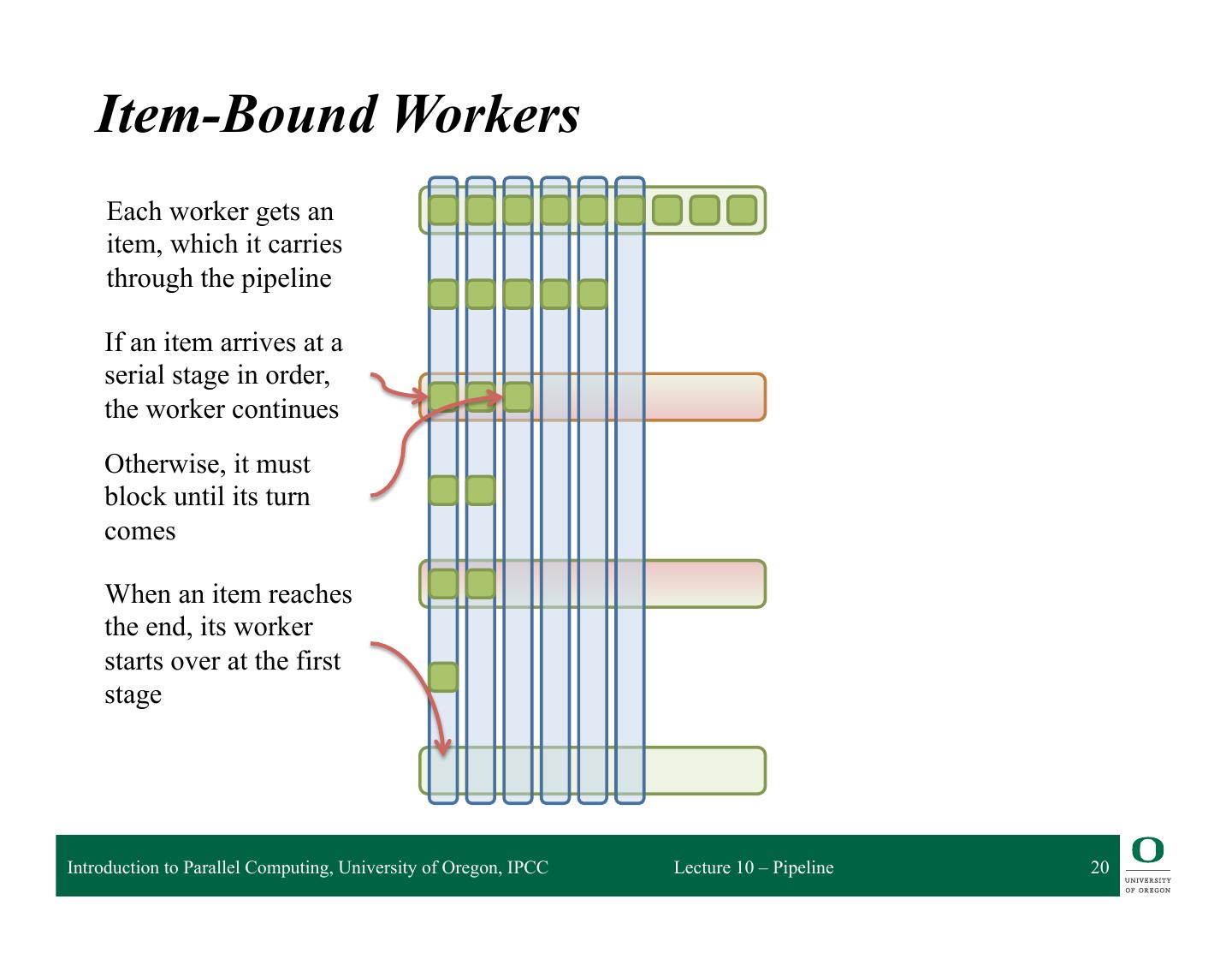
20 . Item-Bound Workers Each worker gets an item, which it carries through the pipeline If an item arrives at a serial stage in order, the worker continues Otherwise, it must block until its turn comes When an item reaches the end, its worker starts over at the first stage Introduction to Parallel Computing, University of Oregon, IPCC Lecture 10 – Pipeline 20 

21 . Implementation Strategies q  Hybrid (as implemented in TBB) ❍  Workers begin as item-bound ❍  When entering a serial stage, the worker checks whether it’s ready to process the item now ◆ If so, the worker continues into the stage ◆ Otherwise, it parks the item, leaving it for another worker, and starts over ❍  When leaving a serial stage, the worker checks for a parked item, spawning a new worker to handle it ❍  Retains good data locality without requiring workers to block at serial stages ❍  No locks needed; works with greedy schedulers Introduction to Parallel Computing, University of Oregon, IPCC Lecture 10 – Pipeline 21 

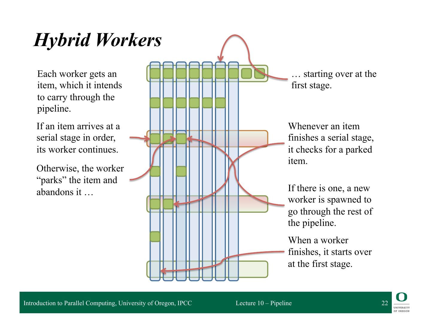
22 . Hybrid Workers Each worker gets an … starting over at the item, which it intends first stage. to carry through the pipeline. If an item arrives at a Whenever an item serial stage in order, finishes a serial stage, its worker continues. it checks for a parked item. Otherwise, the worker “parks” the item and abandons it … If there is one, a new worker is spawned to go through the rest of the pipeline. When a worker finishes, it starts over at the first stage. Introduction to Parallel Computing, University of Oregon, IPCC Lecture 10 – Pipeline 22 

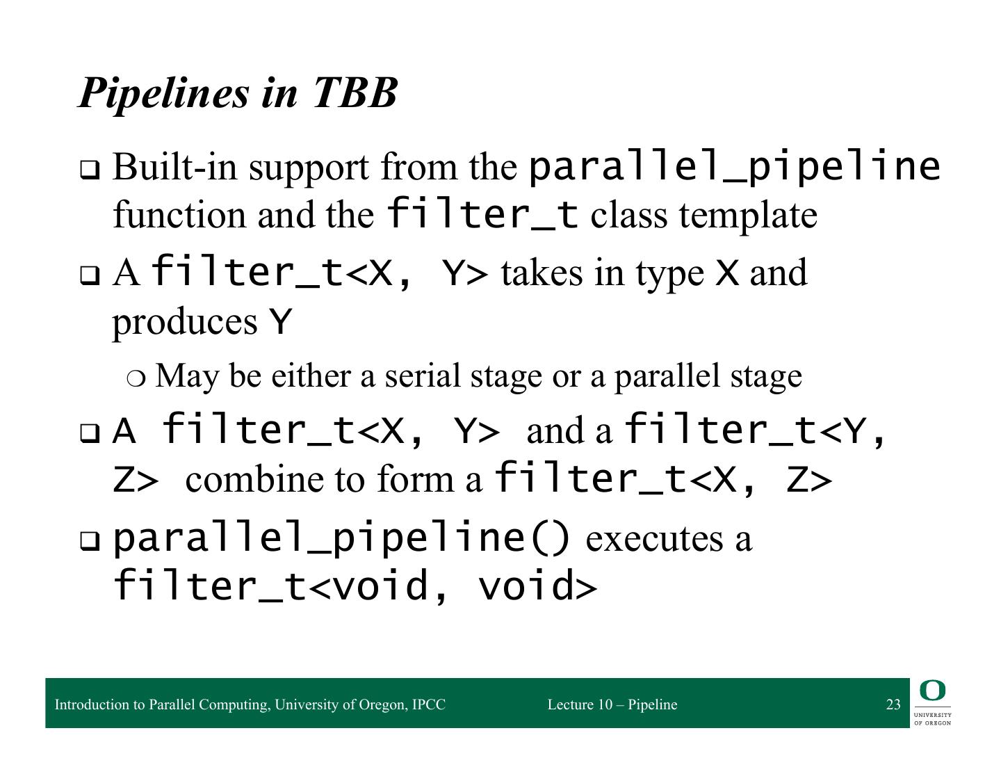
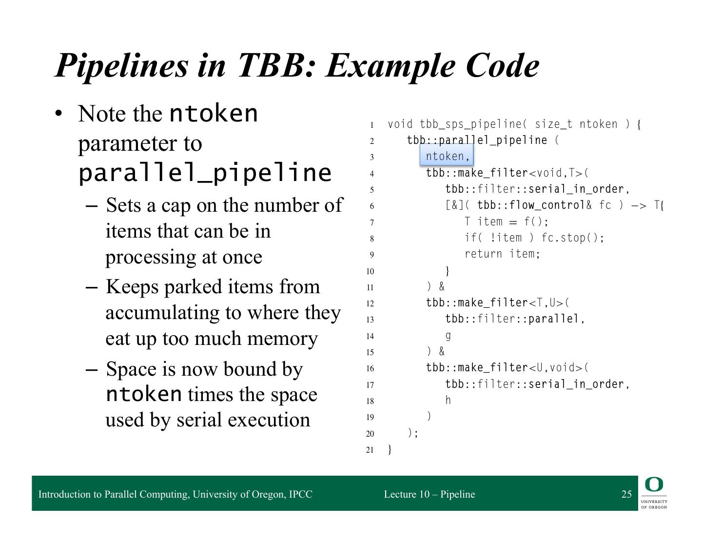
23 . Pipelines in TBB q  Built-insupport from the parallel_pipeline function and the filter_t class template q  A filter_t<X, Y> takes in type X and produces Y ❍  May be either a serial stage or a parallel stage q  A filter_t<X, Y> and a filter_t<Y, Z> combine to form a filter_t<X, Z> q  parallel_pipeline() executes a filter_t<void, void> Introduction to Parallel Computing, University of Oregon, IPCC Lecture 10 – Pipeline 23 

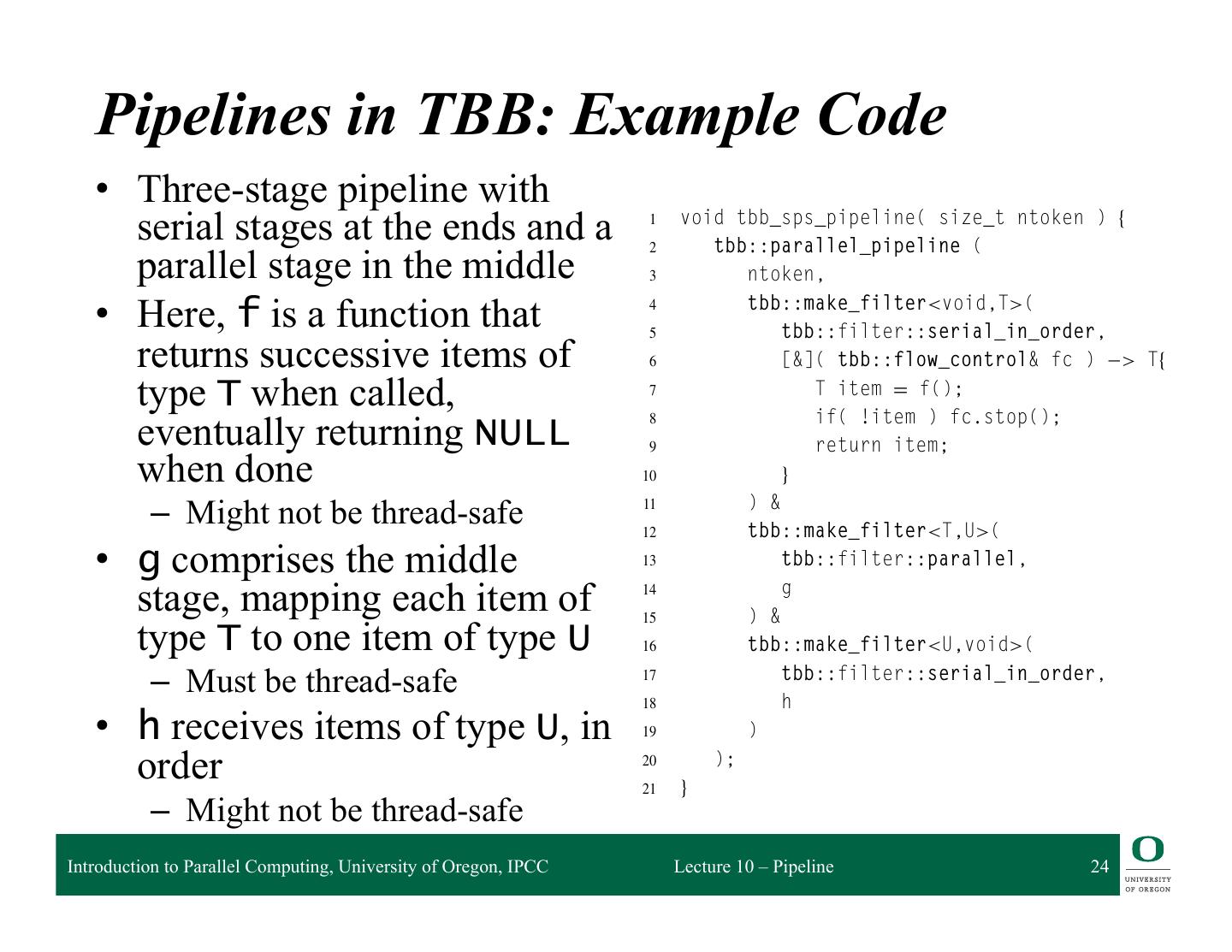
24 . Pipelines in TBB: Example Code 258 CHAPTER 9 Pipeline •  Three-stage pipeline with serial stages at the ends and a 1 2 void tbb_sps_pipeline( size_t ntoken ) { tbb::parallel_pipeline ( parallel stage in the middle 3 ntoken, tbb::make_filter<void,T>( •  Here, f is a function that 4 5 tbb::filter::serial_in_order, returns successive items of 6 [&]( tbb::flow_control& fc ) > T{ type T when called, 7 T item = f(); if( !item ) fc.stop(); eventually returning NULL 8 9 return item; when done 10 } ) & –  Might not be thread-safe 11 12 tbb::make_filter<T,U>( •  g comprises the middle 13 tbb::filter::parallel, stage, mapping each item of 14 15 ) & g type T to one item of type U 16 tbb::make_filter<U,void>( tbb::filter::serial_in_order, –  Must be thread-safe 17 18 h •  h receives items of type U, in 19 ) order 20 21 } ); –  Might not be thread-safe LISTING 9.2 Introduction to Parallel Computing, University of Oregon, IPCC Lecture Pipeline in 10 – Pipeline TBB. It is equivalent to the serial pipeline24in Listing 9.1, e the middle stage processes multiple items in parallel. 

25 . Pipelines in TBB: Example Code 258 CHAPTER 9 Pipeline •  Note the ntoken 1 void tbb_sps_pipeline( size_t ntoken ) { parameter to 2 3 tbb::parallel_pipeline ( ntoken, parallel_pipeline 4 5 tbb::make_filter<void,T>( tbb::filter::serial_in_order, –  Sets a cap on the number of 6 [&]( tbb::flow_control& fc ) > T{ 7 T item = f(); items that can be in 8 if( !item ) fc.stop(); processing at once 9 10 } return item; –  Keeps parked items from 11 ) & 12 tbb::make_filter<T,U>( accumulating to where they 13 tbb::filter::parallel, eat up too much memory 14 15 ) & g –  Space is now bound by 16 tbb::make_filter<U,void>( 17 tbb::filter::serial_in_order, ntoken times the space 18 h used by serial execution 19 20 ); ) 21 } LISTING 9.2 Introduction to Parallel Computing, University of Oregon, IPCC Lecture Pipeline in 10 – Pipeline TBB. It is equivalent to the serial pipeline25in Listing 9.1, e the middle stage processes multiple items in parallel. 

26 . Pipelines in Cilk Plus q  No built-in support for pipelines q  Implementing by hand can be tricky ❍  Can easily fork to move from a serial stage to a parallel stage ❍  But can’t simply join to go from parallel back to serial, since workers must proceed in the correct order ❍  Could gather results from parallel stage in one big list, but this reduces parallelism and may take too much space Introduction to Parallel Computing, University of Oregon, IPCC Lecture 10 – Pipeline 26 

27 . Pipelines in Cilk Plus q  Idea: A reducer can store sub-lists of the results, combining adjacent ones when possible ❍  By itself, this would only implement the one-big-list concept ❍  However, whichever sub-list is farthest left can process items immediately ◆ the list may not even be stored as such; can “add” items to it simply by processing them ❍  Thisway, the serial stage is running as much as possible ❍  Eventually, the leftmost sub-list comprises all items, and thus they are all processed Introduction to Parallel Computing, University of Oregon, IPCC Lecture 10 – Pipeline 27 

28 . Pipelines in Cilk Plus: Monoids q  Each view in the reducer has a sub-list and an is_leftmost flag q  The views are then elements of two monoids* ❍  The usual list-concatenation monoid (a.k.a. the free monoid), storing the items ❍  A monoid* over Booleans that maps x ⊗ y to x, keeping track of which sub-list is leftmost ◆  *Not quite actually a monoid, since a monoid has to have an identity element I for which I ⊗ y is always y ◆  But close enough for our purposes, since the only case that would break is false ⊗ true, and the leftmost view can’t be on the right! q  Combining two views then means concatenating adjacent sub-lists and taking the left is_leftmost Introduction to Parallel Computing, University of Oregon, IPCC Lecture 10 – Pipeline 28 

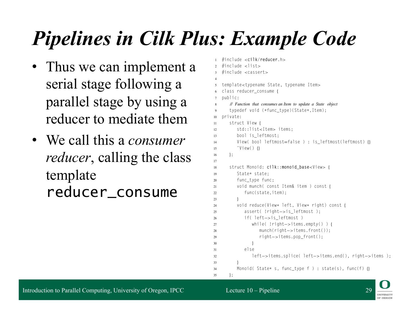
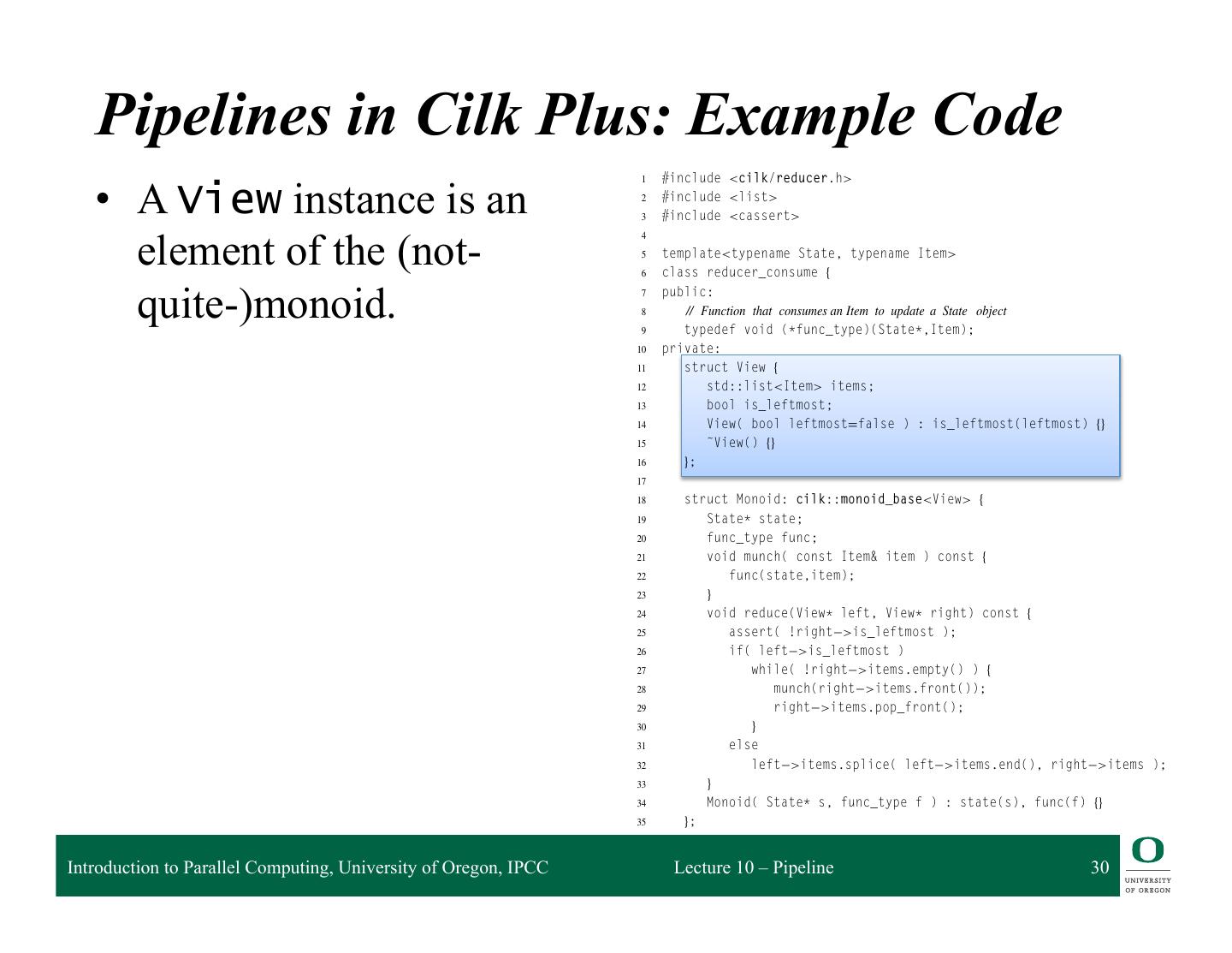
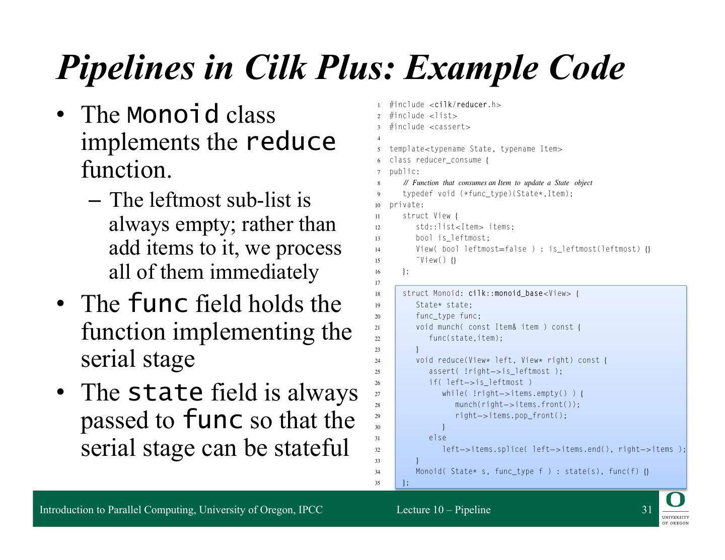
29 . to be deferred. So reducer_consumer joins views using the following rules: • If the left view is leftmost, its list is empty. Process the list of the right view. • Otherwise, concatenate the lists. Pipelines in Cilk Plus: Example Code Listing 9.4 shows the implementation. The list is non-empty only if actual parallelism occurs, only then is there is a non-leftmost view. Section 11.2.1 explains the general mechanics of crea View and Monoid for a cilk::reducer. 1 #include <cilk/reducer.h> •  Thus we can implement a 2 3 #include <list> #include <cassert> serial stage following a 4 5 template<typename State, typename Item> 6 class reducer_consume { parallel stage by using a 7 8 9 public: // Function that consumes an Item to update a State object typedef void (*func_type)(State*,Item); reducer to mediate them 10 11 12 private: struct View { std::list<Item> items; •  We call this a consumer 13 bool is_leftmost; 14 View( bool leftmost=false ) : is_leftmost(leftmost) {} 15 ˜View() {} reducer, calling the class 16 17 18 }; struct Monoid: cilk::monoid_base<View> { template 19 20 State* state; func_type func; 21 void munch( const Item& item ) const { reducer_consume 22 23 } func(state,item); 24 void reduce(View* left, View* right) const { 25 assert( !right >is_leftmost ); 26 if( left >is_leftmost ) 27 while( !right >items.empty() ) { 28 munch(right >items.front()); 29 right >items.pop_front(); 30 } 31 else 32 left >items.splice( left >items.end(), right >items ); 33 } 34 Monoid( State* s, func_type f ) : state(s), func(f) {} 35 }; Introduction to Parallel Computing, University of Oregon, IPCC Lecture 10 – Pipeline 29