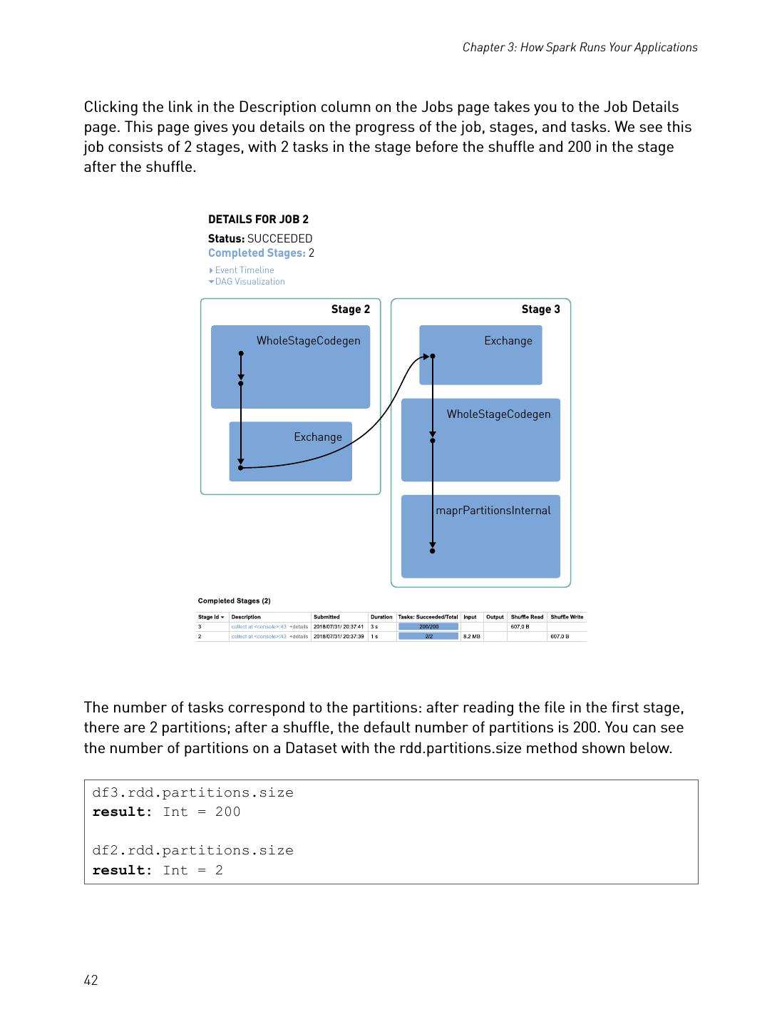
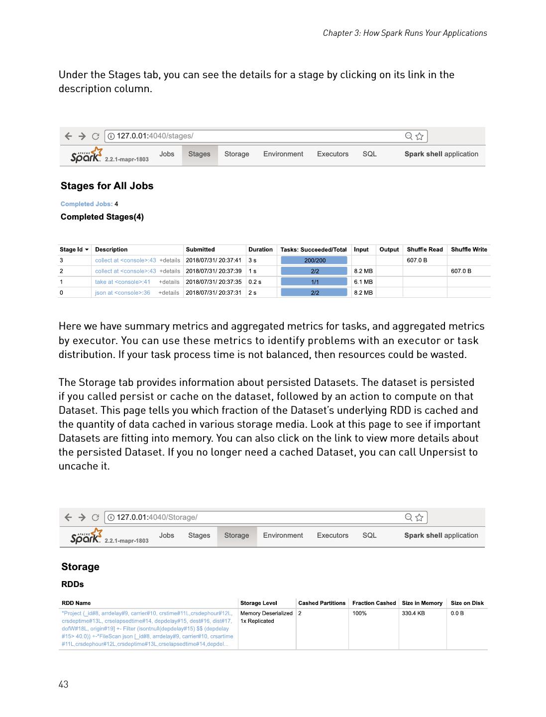
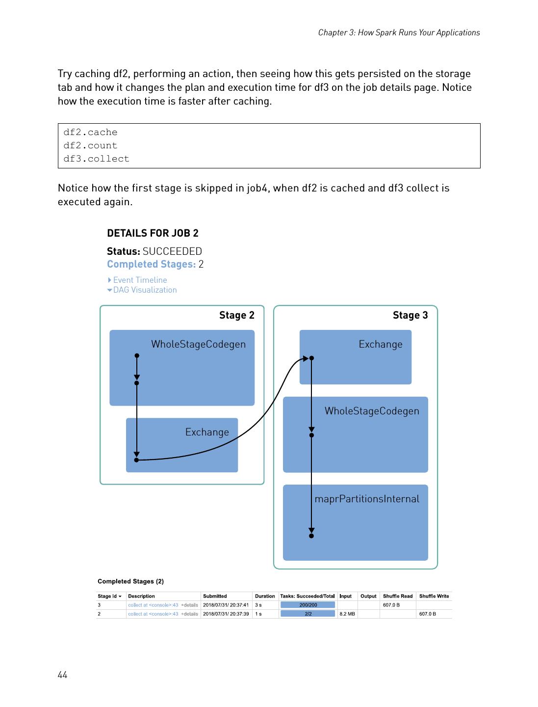
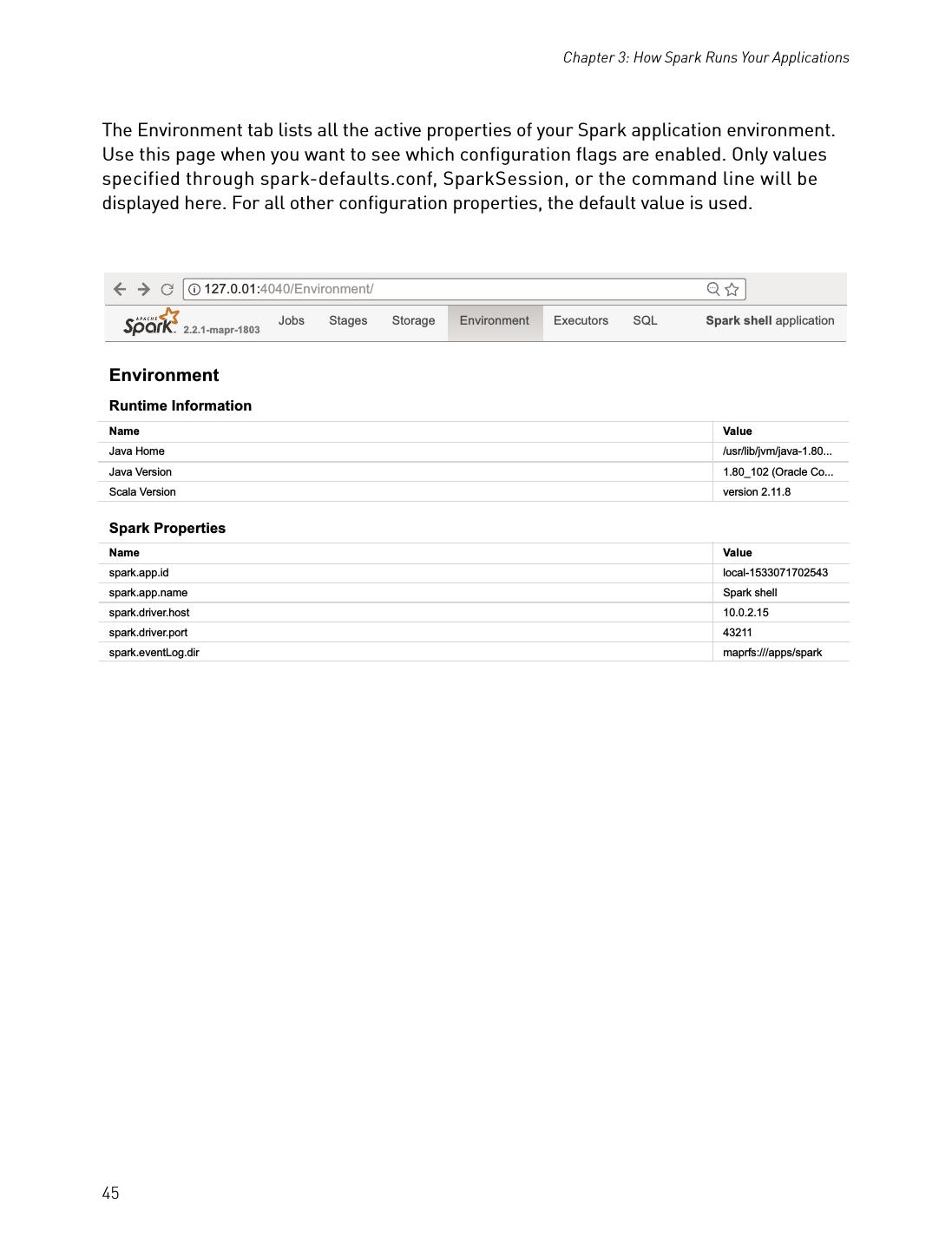
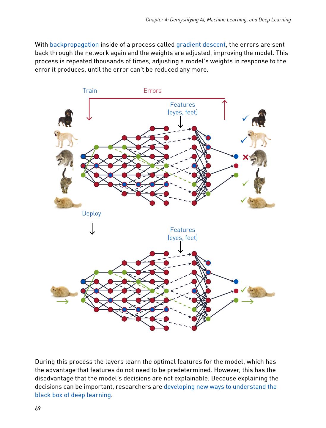
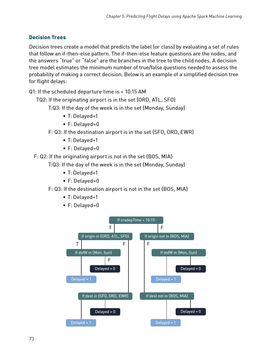
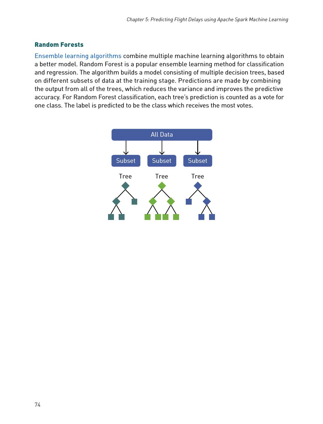
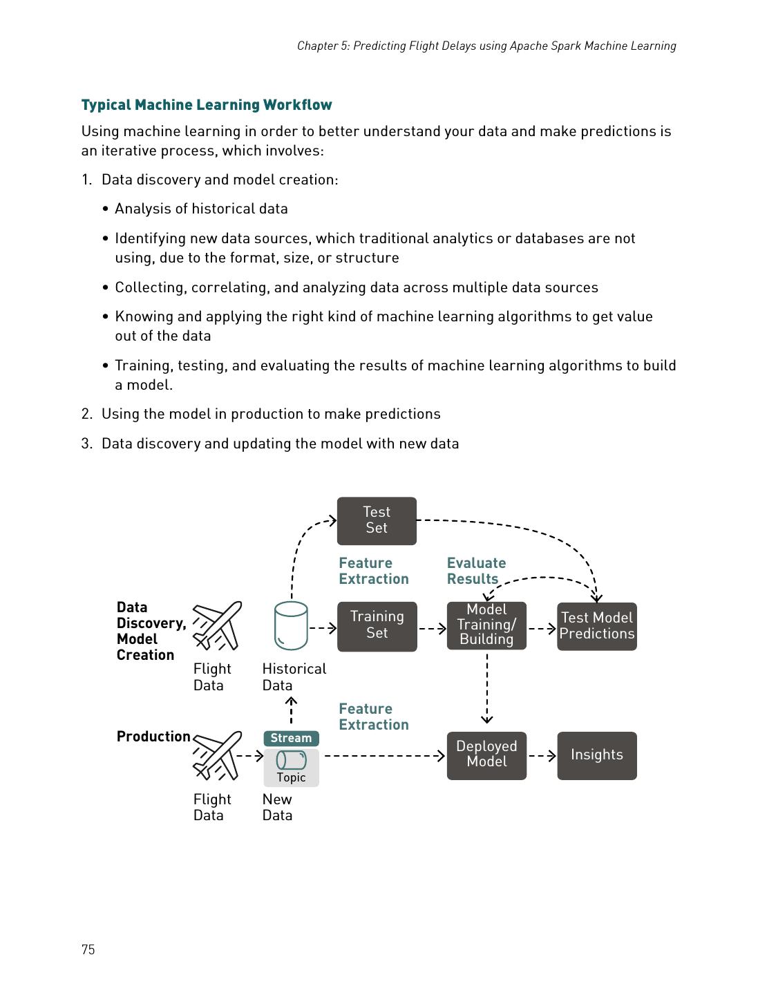
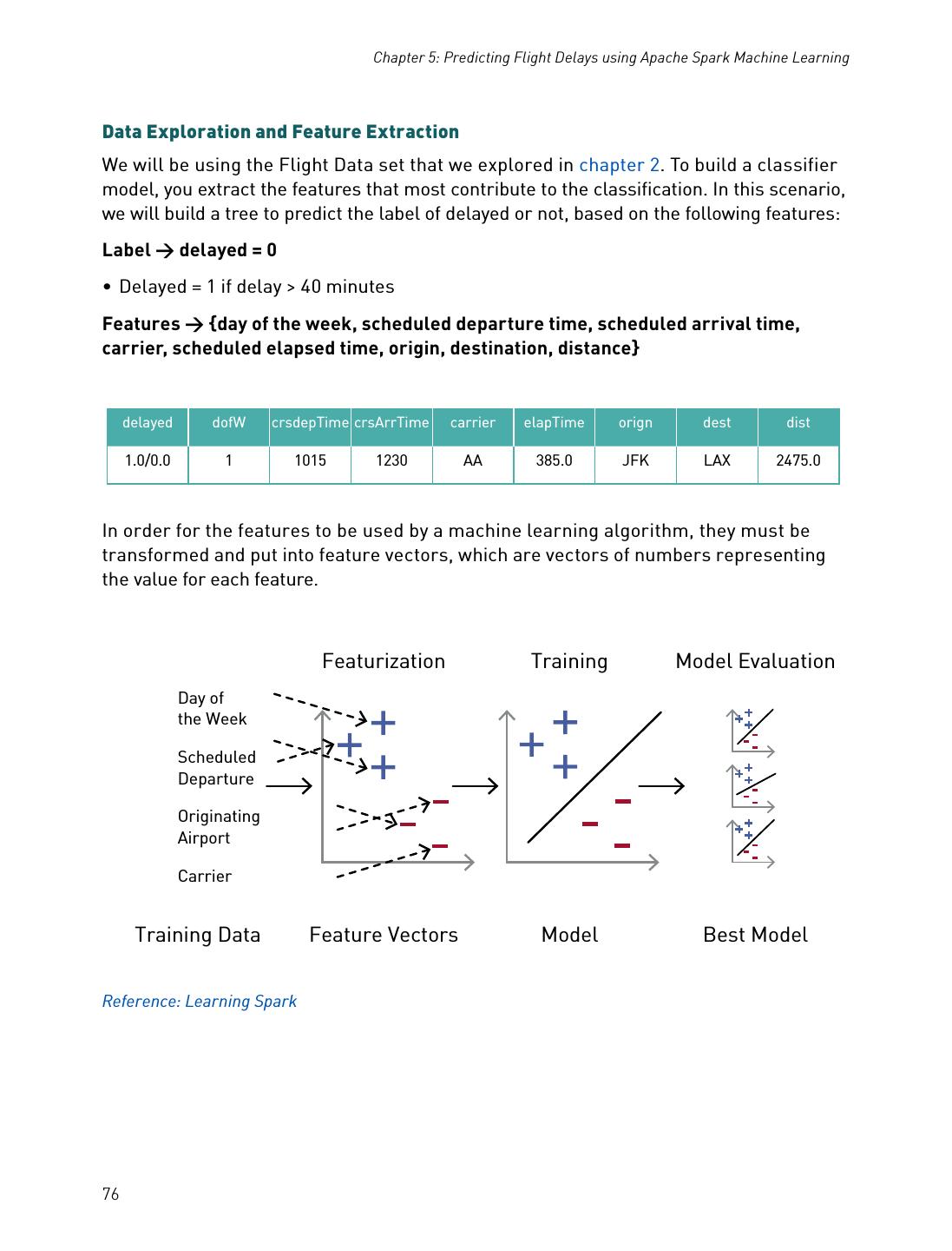
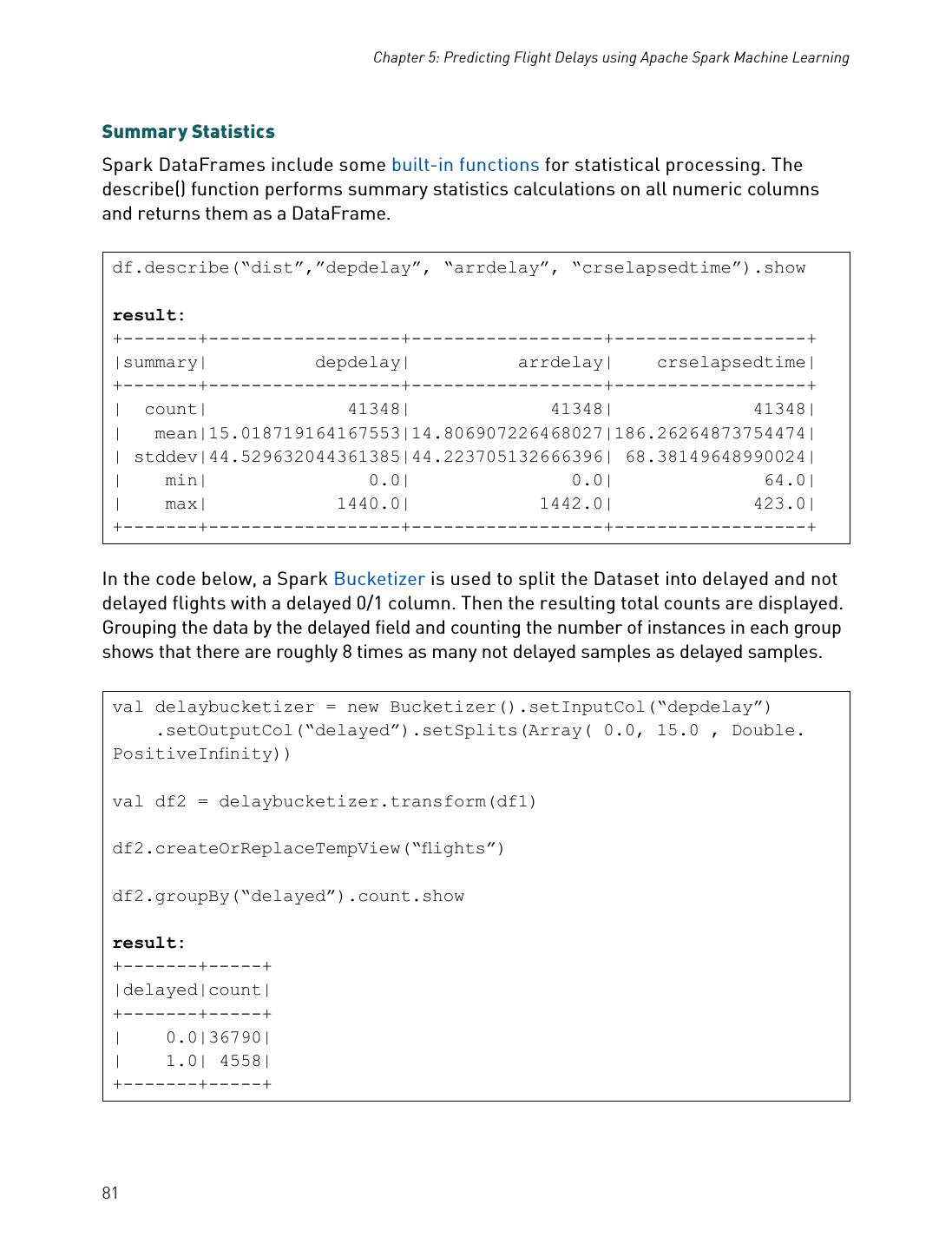
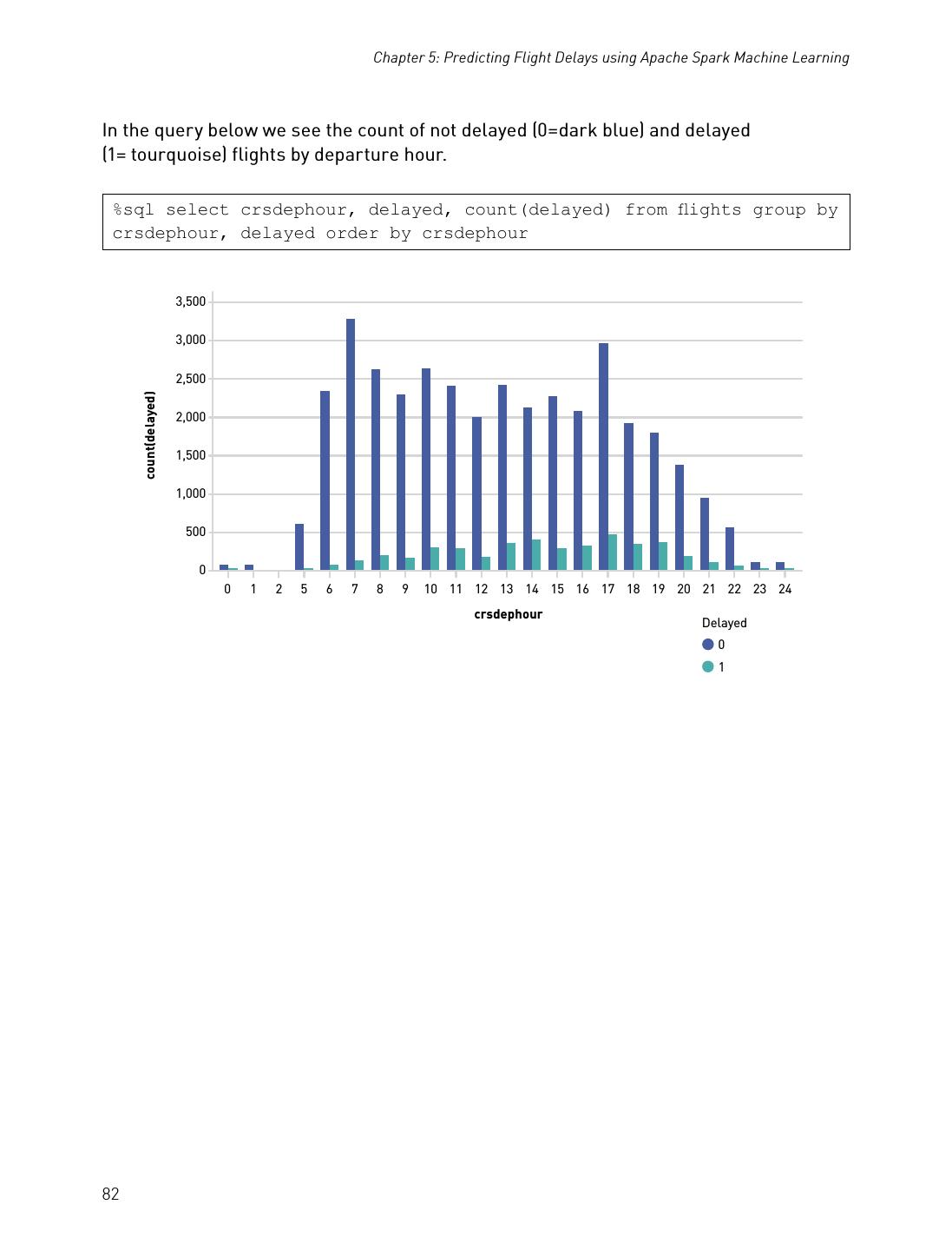
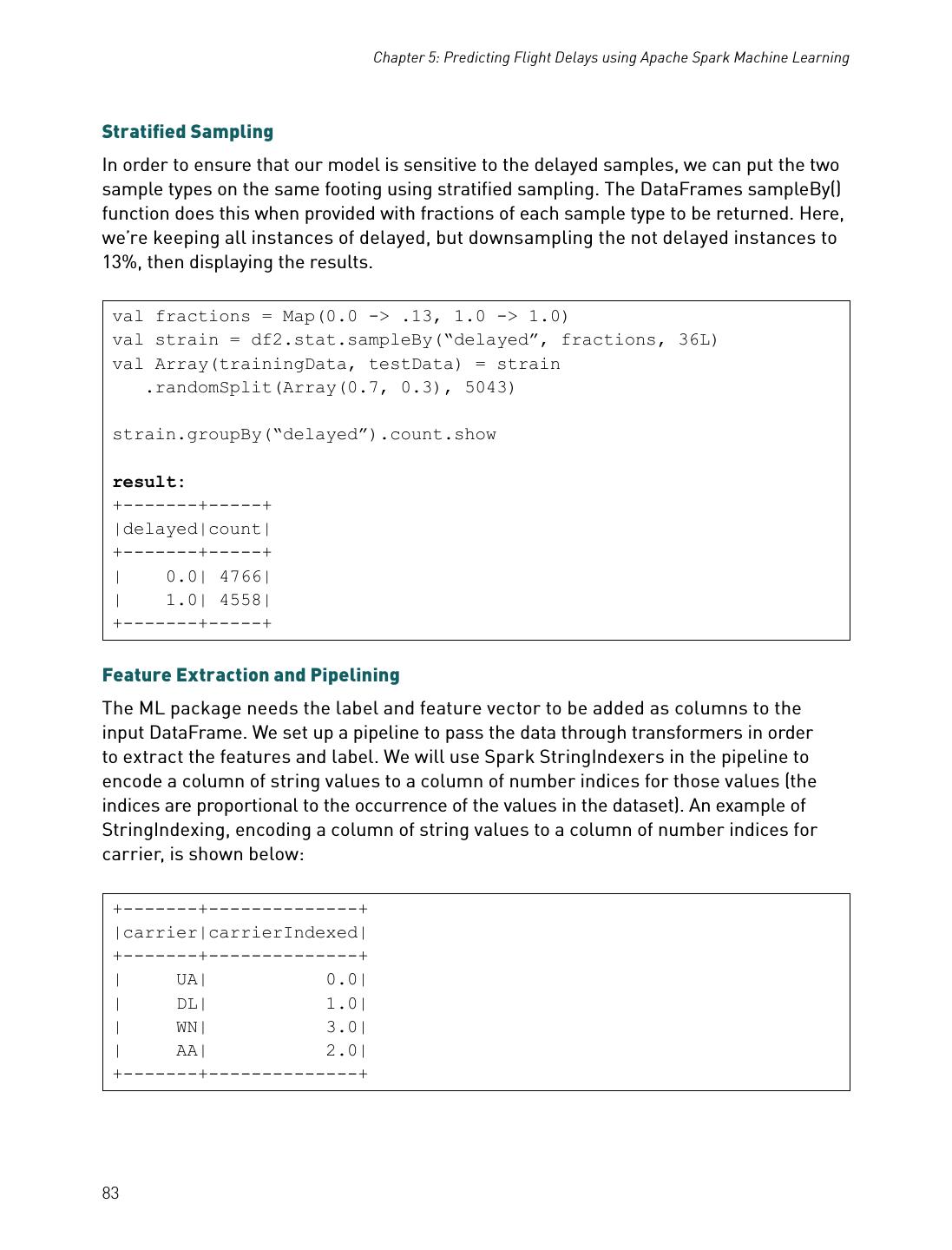
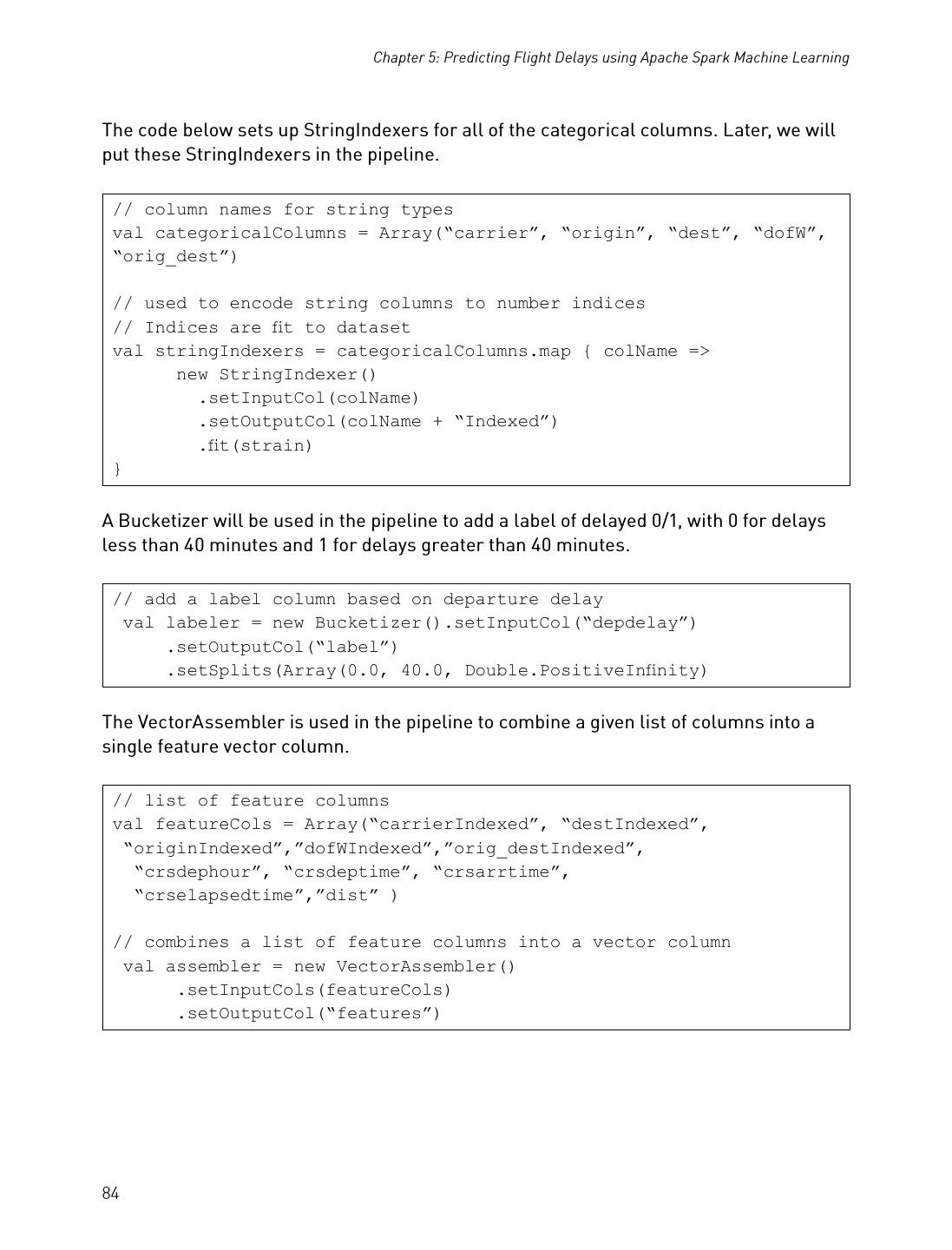
- 快召唤伙伴们来围观吧
- 微博 QQ QQ空间 贴吧
- 文档嵌入链接
- <iframe src="https://www.slidestalk.com/u70/Spark2018eBook?embed" frame border="0" width="640" height="360" scrolling="no" allowfullscreen="true">复制
- 微信扫一扫分享
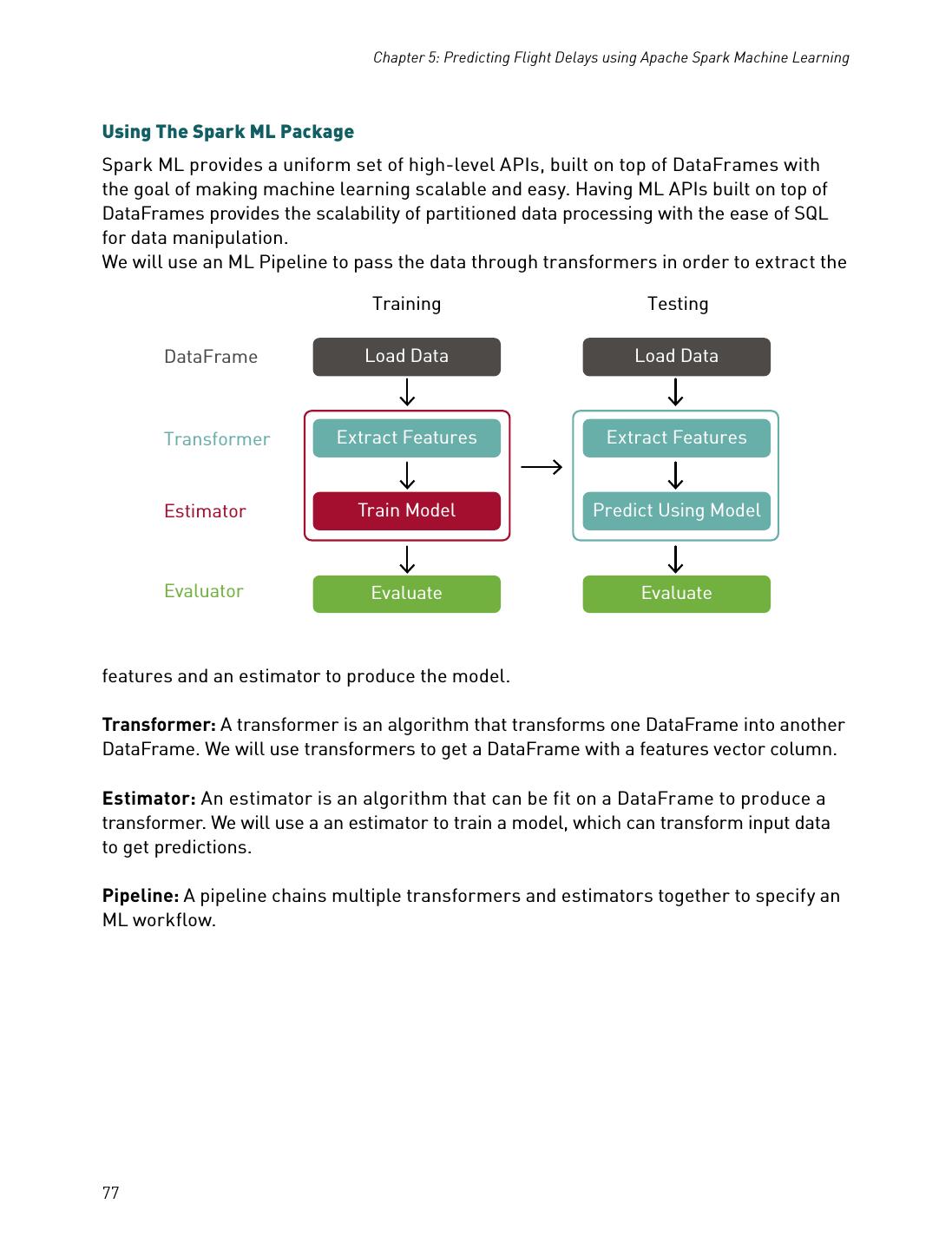
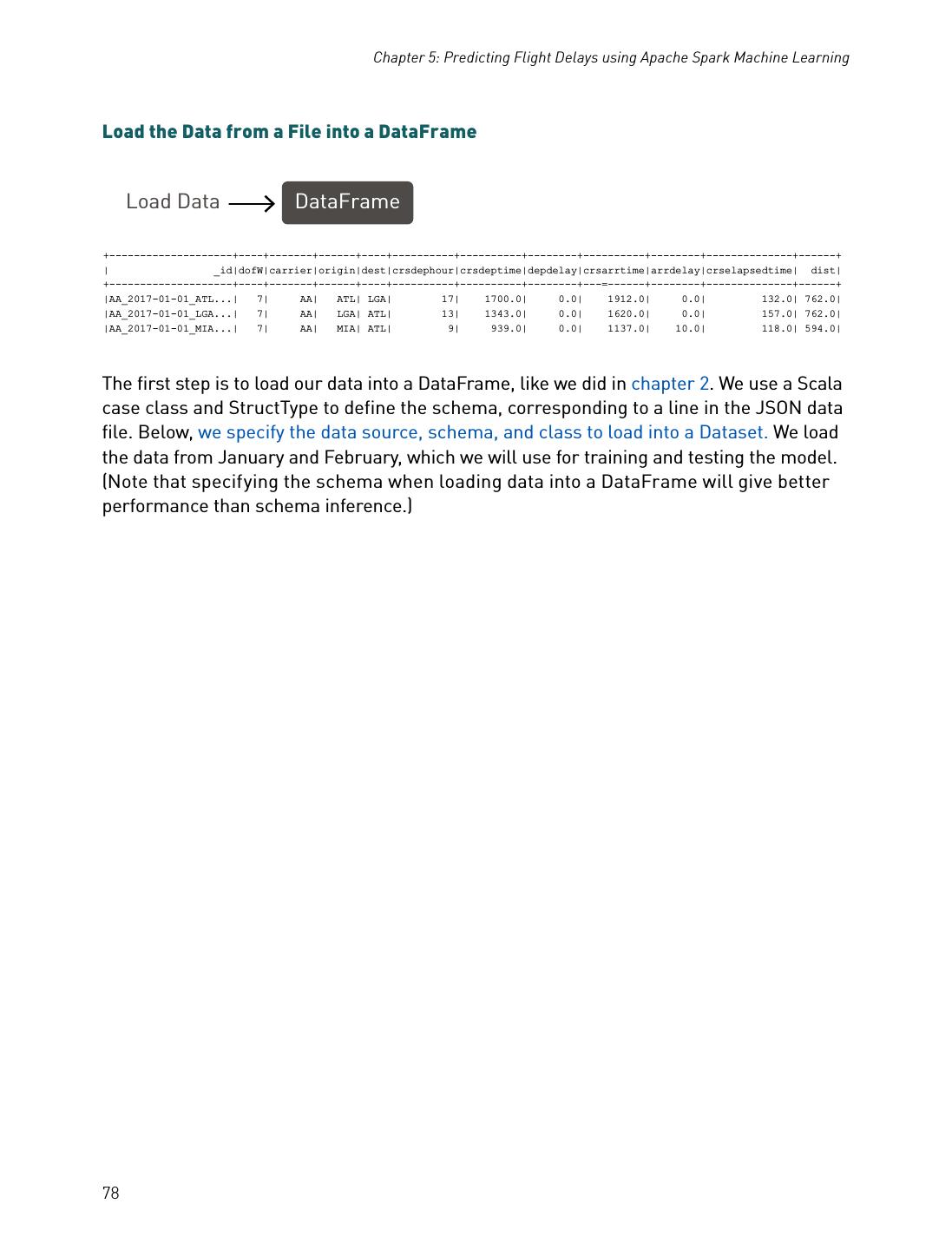
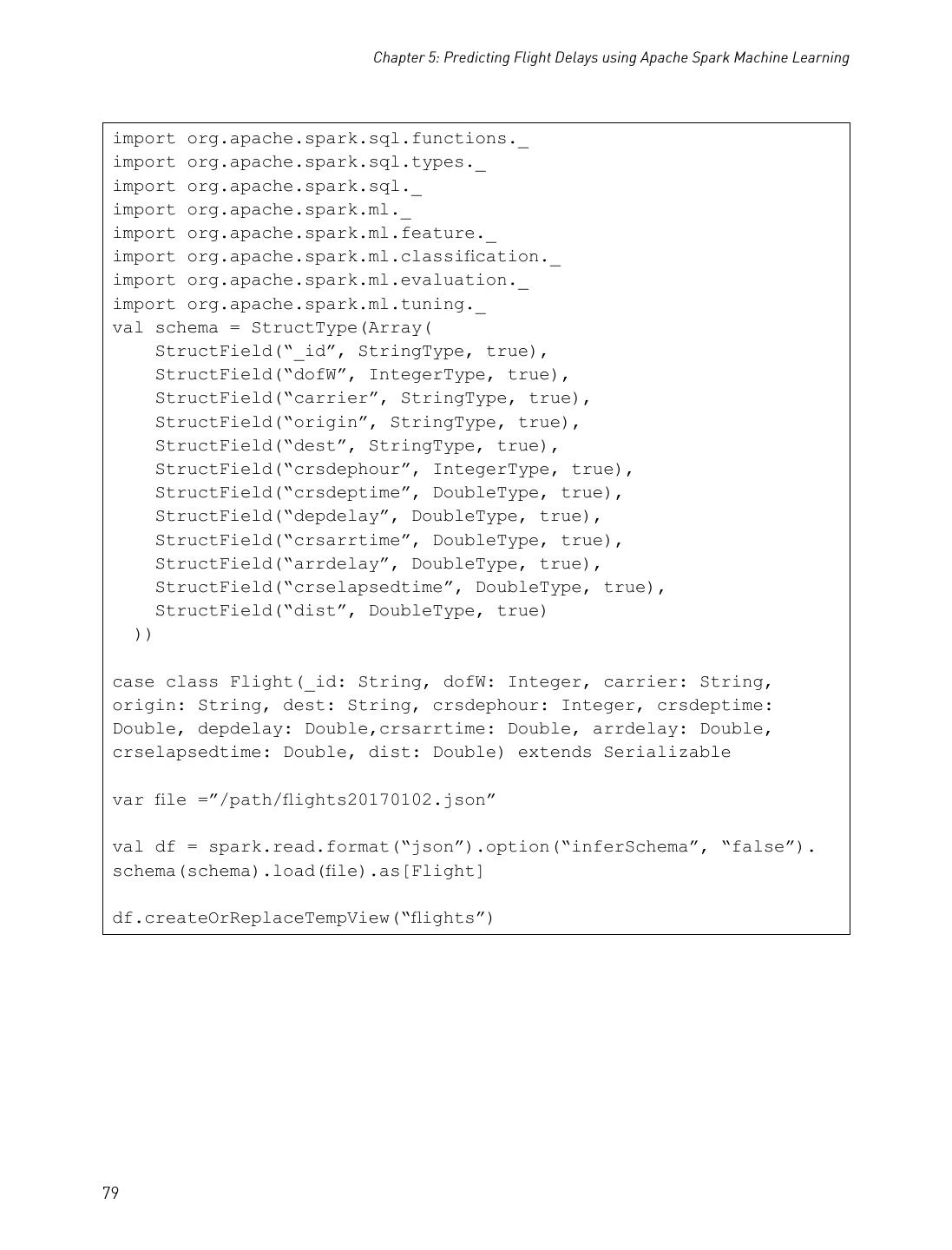
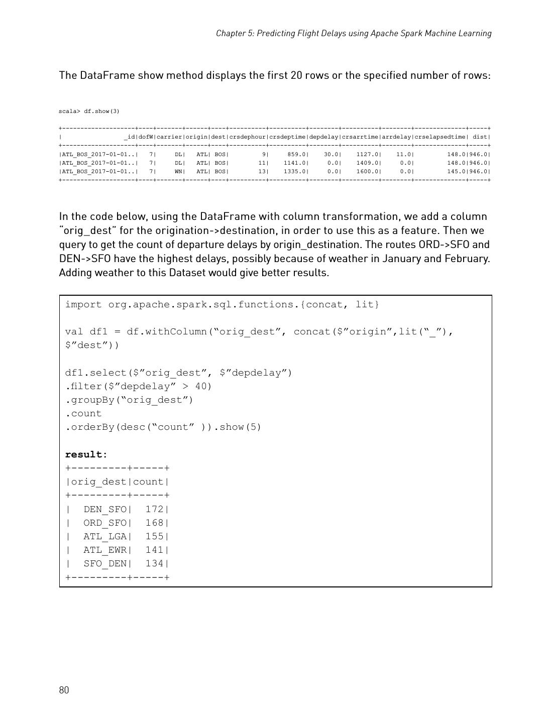
Getting Started with Apache Spark from Inception to Production
展开查看详情
1 . COMPLIMENTS OF EBOOK Getting Started with Apache Spark from Inception to Production Carol McDonald with contribution from Ian Downard
2 .EBOOK Getting Started with Apache Spark from Inception to Production Carol McDonald with contribution from Ian Downard
3 .Getting Started with Apache Spark From Inception to Production By Carol McDonald Copyright © 2018 Carol McDonald, Ian Downard, and MapR Technologies, Inc. All rights reserved. Printed in the United States of America Published by MapR Technologies, Inc. 4555 Great America Parkway, Suite 201 Santa Clara, CA 95054 October 2018: Second Edition Revision History for the First Edition 2015-09-01: First release Apache, Apache Spark, Apache Hadoop, Spark, and Hadoop are trademarks of The Apache Software Foundation. Used with permission. No endorsement by The Apache Software Foundation is implied by the use of these marks. While every precaution has been taken in the preparation of this book, the publisher and authors assume no responsibility for errors or omissions or for damages resulting from the use of the information contained herein.
4 .Table of Contents Chapter 1 Spark 101: What It Is, What It Does, and Why It Matters 5 Chapter 2 Datasets, DataFrames, and Spark SQL 13 Chapter 3 How Spark Runs Your Applications 30 Chapter 4 Demystifying AI, Machine Learning, and Deep Learning 47 Chapter 5 Predicting Flight Delays Using Apache Spark Machine Learning 71 Chapter 6 Cluster Analysis on Uber Event Data to Detect and Visualize Popular 94 Uber Locations Chapter 7 Real-Time Analysis of Popular Uber Locations Using Apache APIs: 110 Spark Structured Streaming, Machine Learning, Kafka, and MapR-DB Chapter 8 Predicting Forest Fire Locations with K-Means in Spark 135 Chapter 9 Using Apache Spark GraphFrames to Analyze Flight Delays 144 and Distances Chapter 10 Tips and Best Practices to Take Advantage of Spark 2.x 172 Appendix 192
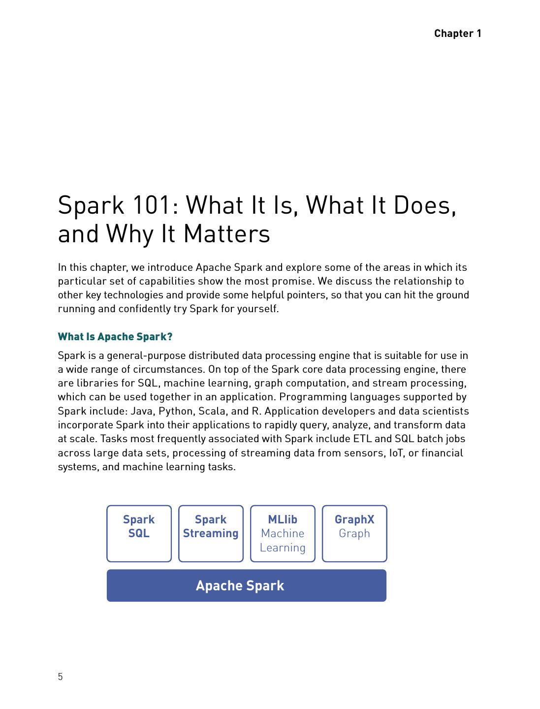
5 . Chapter 1 Spark 101: What It Is, What It Does, and Why It Matters In this chapter, we introduce Apache Spark and explore some of the areas in which its particular set of capabilities show the most promise. We discuss the relationship to other key technologies and provide some helpful pointers, so that you can hit the ground running and confidently try Spark for yourself. What Is Apache Spark? Spark is a general-purpose distributed data processing engine that is suitable for use in a wide range of circumstances. On top of the Spark core data processing engine, there are libraries for SQL, machine learning, graph computation, and stream processing, which can be used together in an application. Programming languages supported by Spark include: Java, Python, Scala, and R. Application developers and data scientists incorporate Spark into their applications to rapidly query, analyze, and transform data at scale. Tasks most frequently associated with Spark include ETL and SQL batch jobs across large data sets, processing of streaming data from sensors, IoT, or financial systems, and machine learning tasks. Spark Spark MLIib GraphX SQL Streaming Machine Graph Learning Apache Spark 5
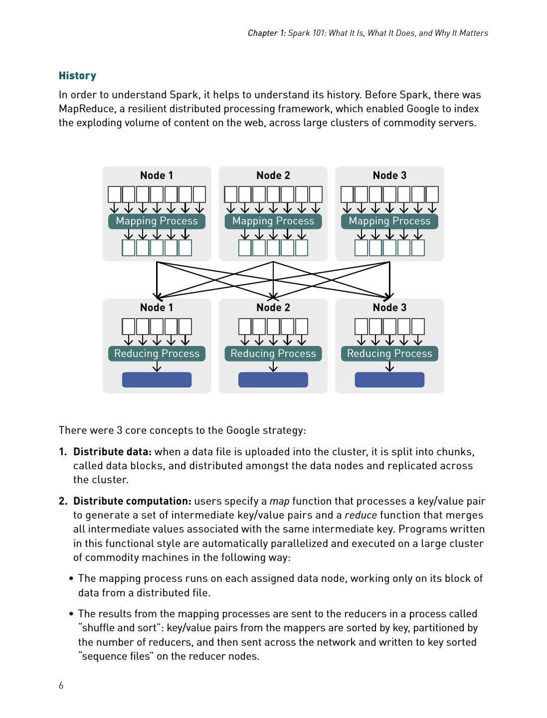
6 . Chapter 1: Spark 101: What It Is, What It Does, and Why It Matters History In order to understand Spark, it helps to understand its history. Before Spark, there was MapReduce, a resilient distributed processing framework, which enabled Google to index the exploding volume of content on the web, across large clusters of commodity servers. Node 1 Node 2 Node 3 Mapping Process Mapping Process Mapping Process Node 1 Node 2 Node 3 Reducing Process Reducing Process Reducing Process There were 3 core concepts to the Google strategy: 1. Distribute data: when a data file is uploaded into the cluster, it is split into chunks, called data blocks, and distributed amongst the data nodes and replicated across the cluster. 2. Distribute computation: users specify a map function that processes a key/value pair to generate a set of intermediate key/value pairs and a reduce function that merges all intermediate values associated with the same intermediate key. Programs written in this functional style are automatically parallelized and executed on a large cluster of commodity machines in the following way: • The mapping process runs on each assigned data node, working only on its block of data from a distributed file. • The results from the mapping processes are sent to the reducers in a process called “shuffle and sort”: key/value pairs from the mappers are sorted by key, partitioned by the number of reducers, and then sent across the network and written to key sorted “sequence files” on the reducer nodes. 6
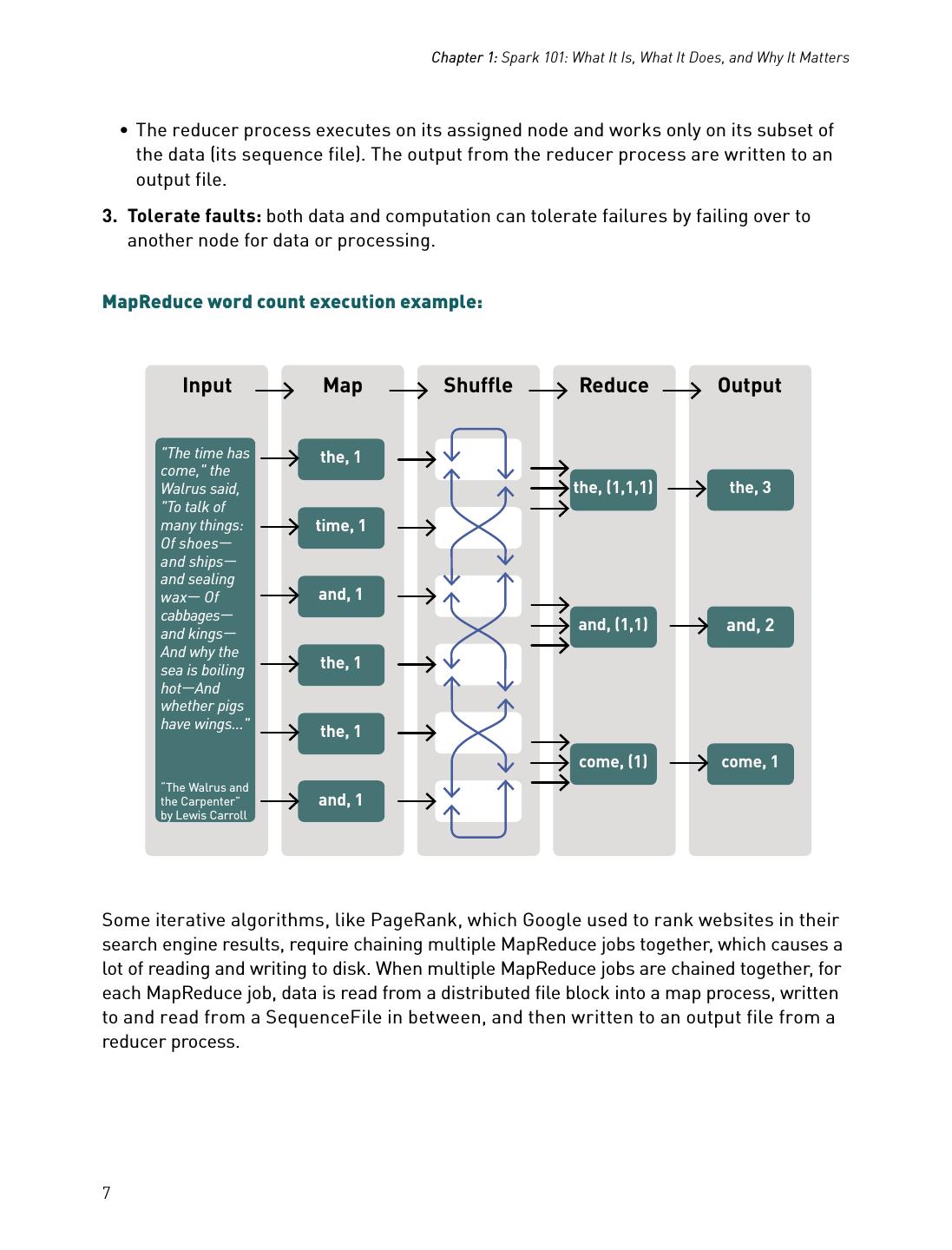
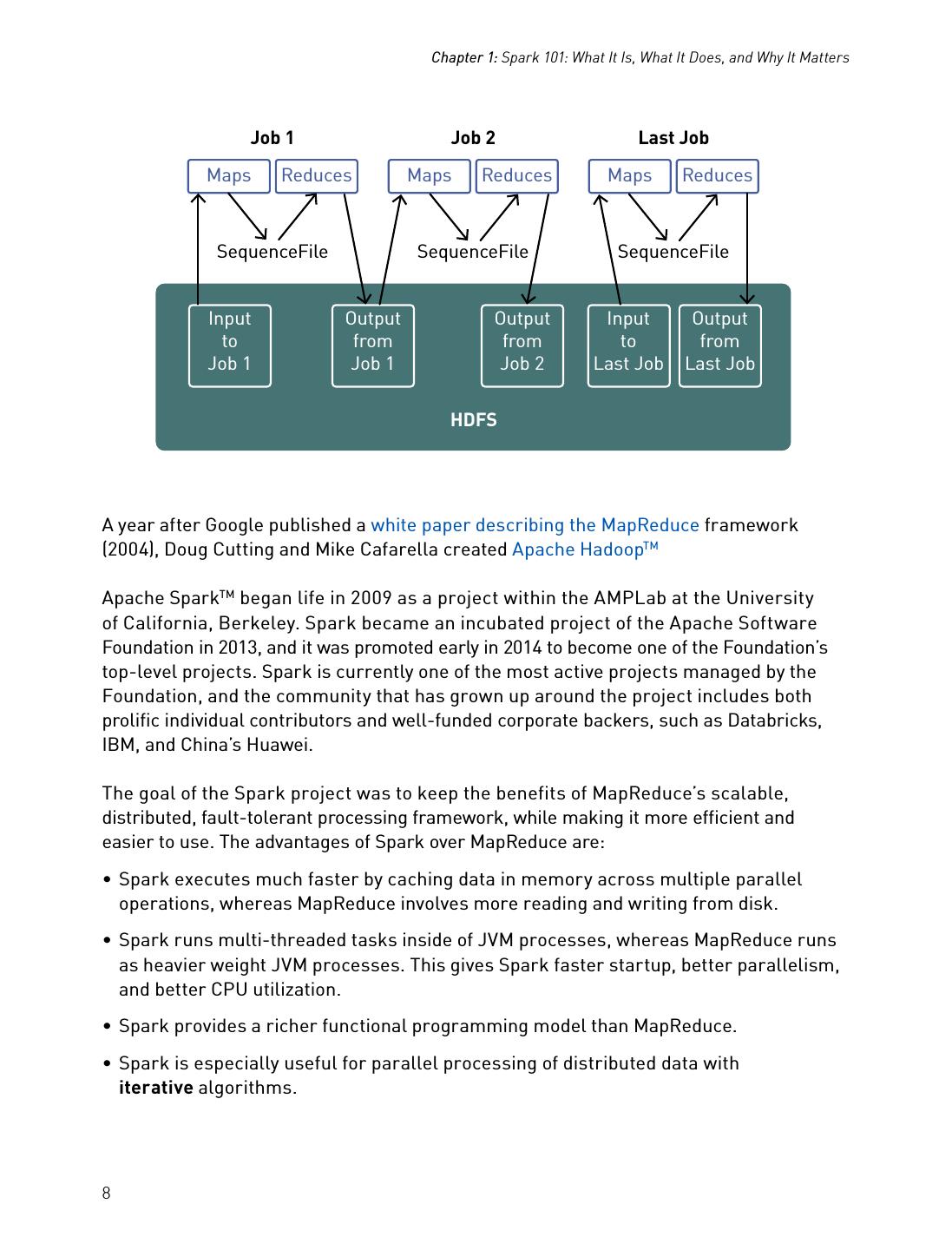
7 . Chapter 1: Spark 101: What It Is, What It Does, and Why It Matters • The reducer process executes on its assigned node and works only on its subset of the data (its sequence file). The output from the reducer process are written to an output file. 3. Tolerate faults: both data and computation can tolerate failures by failing over to another node for data or processing. MapReduce word count execution example: Input Map Shuffle Reduce Output "The time has the, 1 come," the Walrus said, the, (1,1,1) the, 3 "To talk of many things: time, 1 Of shoes— and ships— and sealing wax— Of and, 1 cabbages— and kings— and, (1,1) and, 2 And why the sea is boiling the, 1 hot—And whether pigs have wings..." the, 1 come, (1) come, 1 “The Walrus and the Carpenter” and, 1 by Lewis Carroll Some iterative algorithms, like PageRank, which Google used to rank websites in their search engine results, require chaining multiple MapReduce jobs together, which causes a lot of reading and writing to disk. When multiple MapReduce jobs are chained together, for each MapReduce job, data is read from a distributed file block into a map process, written to and read from a SequenceFile in between, and then written to an output file from a reducer process. 7
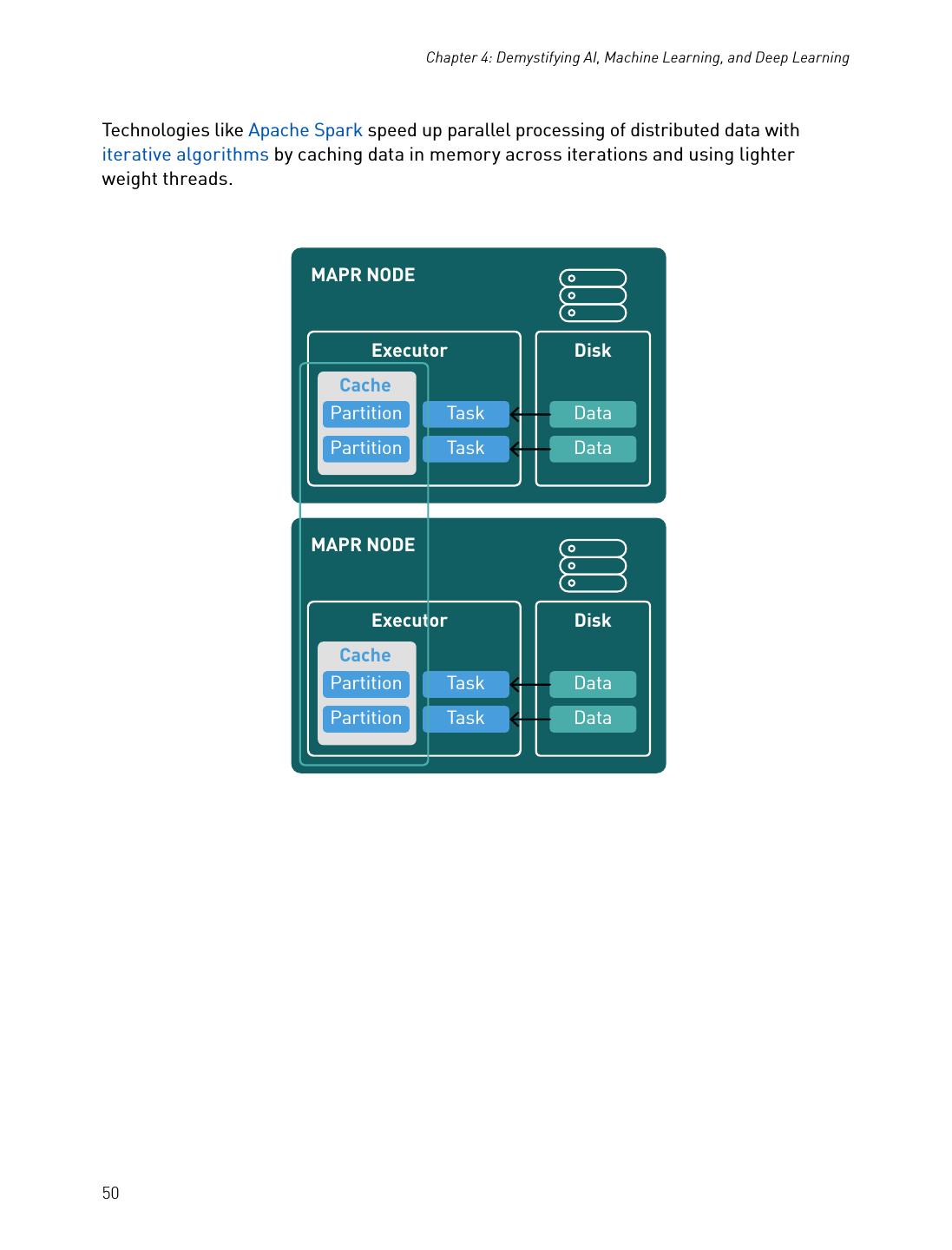
8 . Chapter 1: Spark 101: What It Is, What It Does, and Why It Matters Job 1 Job 2 Last Job Maps Reduces Maps Reduces Maps Reduces SequenceFile SequenceFile SequenceFile Input Output Output Input Output to from from to from Job 1 Job 1 Job 2 Last Job Last Job HDFS A year after Google published a white paper describing the MapReduce framework (2004), Doug Cutting and Mike Cafarella created Apache HadoopTM Apache SparkTM began life in 2009 as a project within the AMPLab at the University of California, Berkeley. Spark became an incubated project of the Apache Software Foundation in 2013, and it was promoted early in 2014 to become one of the Foundation’s top-level projects. Spark is currently one of the most active projects managed by the Foundation, and the community that has grown up around the project includes both prolific individual contributors and well-funded corporate backers, such as Databricks, IBM, and China’s Huawei. The goal of the Spark project was to keep the benefits of MapReduce’s scalable, distributed, fault-tolerant processing framework, while making it more efficient and easier to use. The advantages of Spark over MapReduce are: • Spark executes much faster by caching data in memory across multiple parallel operations, whereas MapReduce involves more reading and writing from disk. • Spark runs multi-threaded tasks inside of JVM processes, whereas MapReduce runs as heavier weight JVM processes. This gives Spark faster startup, better parallelism, and better CPU utilization. • Spark provides a richer functional programming model than MapReduce. • Spark is especially useful for parallel processing of distributed data with iterative algorithms. 8
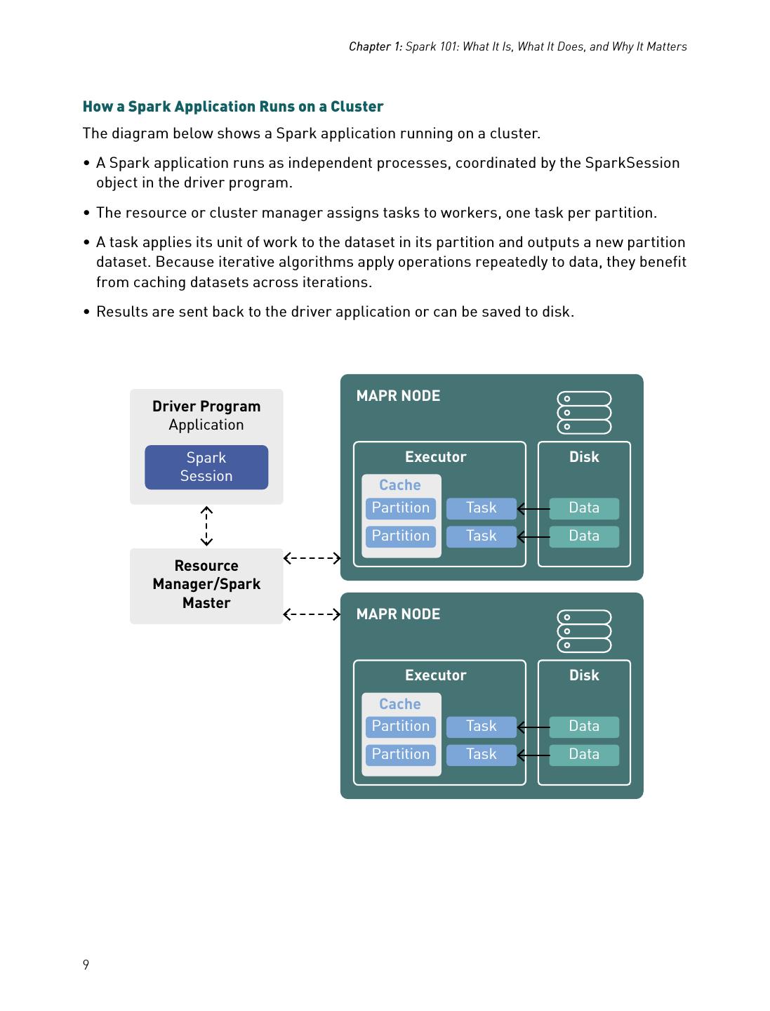
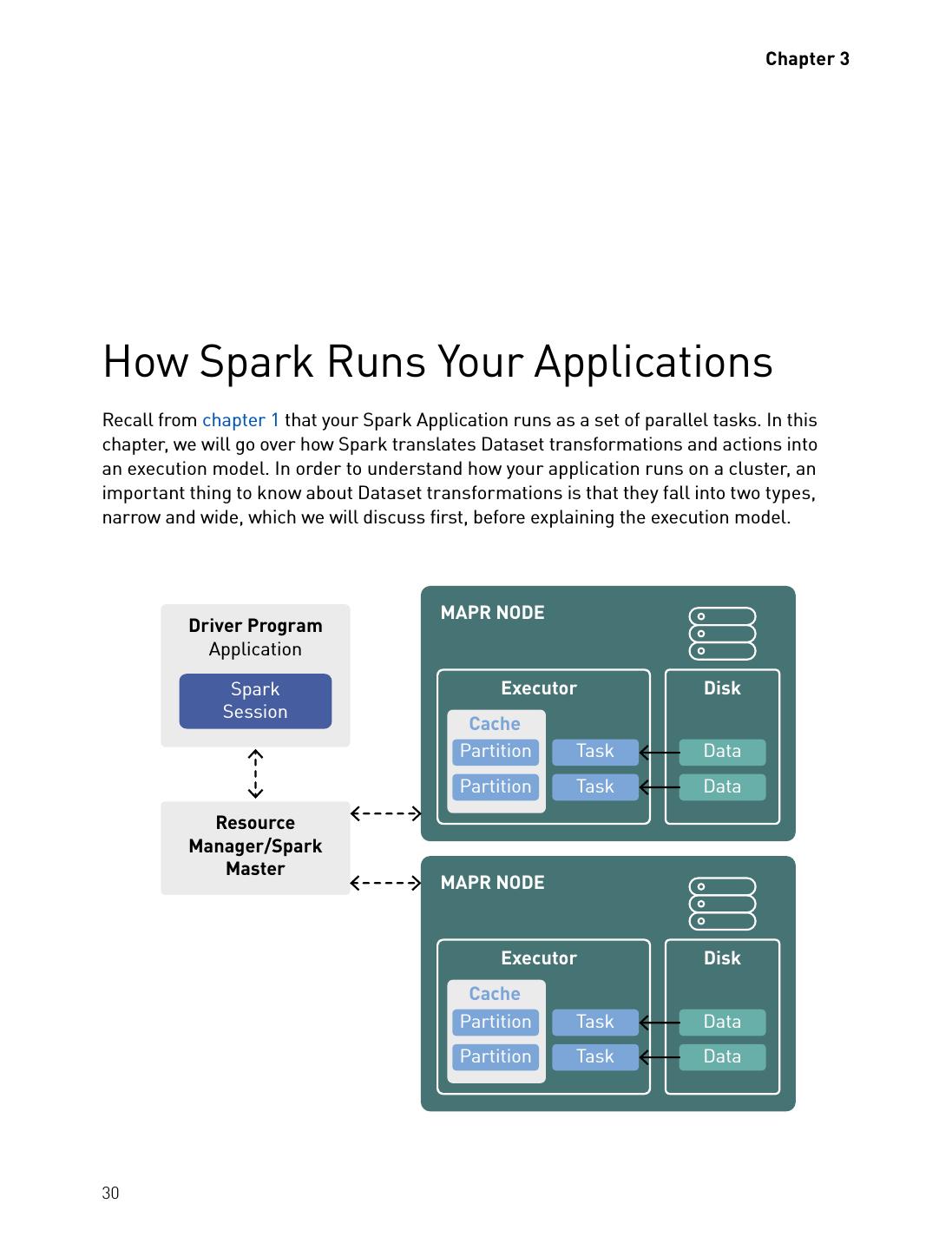
9 . Chapter 1: Spark 101: What It Is, What It Does, and Why It Matters How a Spark Application Runs on a Cluster The diagram below shows a Spark application running on a cluster. • A Spark application runs as independent processes, coordinated by the SparkSession object in the driver program. • The resource or cluster manager assigns tasks to workers, one task per partition. • A task applies its unit of work to the dataset in its partition and outputs a new partition dataset. Because iterative algorithms apply operations repeatedly to data, they benefit from caching datasets across iterations. • Results are sent back to the driver application or can be saved to disk. MAPR NODE Driver Program Application Spark Executor Disk Session Cache Partition Task Data Partition Task Data Resource Manager/Spark Master MAPR NODE Executor Disk Cache Partition Task Data Partition Task Data 9
10 . Chapter 1: Spark 101: What It Is, What It Does, and Why It Matters Spark supports the following resource/cluster managers: Spark Standalone – a simple cluster manager included with Spark Apache Mesos – a general cluster manager that can also run Hadoop applications Apache Hadoop YARN – the resource manager in Hadoop 2 Kubernetes – an open source system for automating deployment, scaling, and management of containerized applications Spark also has a local mode, where the driver and executors run as threads on your computer instead of a cluster, which is useful for developing your applications from a personal computer. What Does Spark Do? Spark is capable of handling several petabytes of data at a time, distributed across a cluster of thousands of cooperating physical or virtual servers. It has an extensive set of developer libraries and APIs and supports languages such as Java, Python, R, and Scala; its flexibility makes it well-suited for a range of use cases. Spark is often used with distributed data data stores such as MapR-XD, Hadoop’s HDFS, and Amazon’s S3, with popular NoSQL databases such as MapR-DB, Apache HBase, Apache Cassandra, and MongoDB, and with distributed messaging stores such as MapR-ES and Apache Kafka. Typical use cases include: Stream processing: From log files to sensor data, application developers are increasingly having to cope with “streams” of data. This data arrives in a steady stream, often from multiple sources simultaneously. While it is certainly feasible to store these data streams on disk and analyze them retrospectively, it can sometimes be sensible or important to process and act upon the data as it arrives. Streams of data related to financial transactions, for example, can be processed in real time to identify – and refuse – potentially fraudulent transactions. Machine learning: As data volumes grow, machine learning approaches become more feasible and increasingly accurate. Software can be trained to identify and act upon triggers within well-understood data sets before applying the same solutions to new and unknown data. Spark’s ability to store data in memory and rapidly run repeated queries makes it a good choice for training machine learning algorithms. Running broadly similar queries again and again, at scale, significantly reduces the time required to go through a set of possible solutions in order to find the most efficient algorithms. 10
11 . Chapter 1: Spark 101: What It Is, What It Does, and Why It Matters Interactive analytics: Rather than running pre-defined queries to create static dashboards of sales or production line productivity or stock prices, business analysts and data scientists want to explore their data by asking a question, viewing the result, and then either altering the initial question slightly or drilling deeper into results. This interactive query process requires systems such as Spark that are able to respond and adapt quickly. Data integration: Data produced by different systems across a business is rarely clean or consistent enough to simply and easily be combined for reporting or analysis. Extract, transform, and load (ETL) processes are often used to pull data from different systems, clean and standardize it, and then load it into a separate system for analysis. Spark (and Hadoop) are increasingly being used to reduce the cost and time required for this ETL process. Who Uses Spark? A wide range of technology vendors have been quick to support Spark, recognizing the opportunity to extend their existing big data products into areas where Spark delivers real value, such as interactive querying and machine learning. Well-known companies such as IBM and Huawei have invested significant sums in the technology, and a growing number of startups are building businesses that depend in whole or in part upon Spark. For example, in 2013 the Berkeley team responsible for creating Spark founded Databricks, which provides a hosted end-to-end data platform powered by Spark. The company is well-funded, having received $47 million across two rounds of investment in 2013 and 2014, and Databricks employees continue to play a prominent role in improving and extending the open source code of the Apache Spark project. The major Hadoop vendors, including MapR, Cloudera, and Hortonworks, have all moved to support YARN-based Spark alongside their existing products, and each vendor is working to add value for its customers. Elsewhere, IBM, Huawei, and others have all made significant investments in Apache Spark, integrating it into their own products and contributing enhancements and extensions back to the Apache project. Web-based companies, like Chinese search engine Baidu, e-commerce operation Taobao, and social networking company Tencent, all run Spark-based operations at scale, with Tencent’s 800 million active users reportedly generating over 700 TB of data per day for processing on a cluster of more than 8,000 compute nodes. In addition to those web-based giants, pharmaceutical company Novartis depends upon Spark to reduce the time required to get modeling data into the hands of researchers, while ensuring that ethical and contractual safeguards are maintained. 11
12 . Chapter 1: Spark 101: What It Is, What It Does, and Why It Matters What Sets Spark Apart? There are many reasons to choose Spark, but three are key: Simplicity: Spark’s capabilities are accessible via a set of rich APIs, all designed specifically for interacting quickly and easily with data at scale. These APIs are well- documented and structured in a way that makes it straightforward for data scientists and application developers to quickly put Spark to work. Speed: Spark is designed for speed, operating both in memory and on disk. Using Spark, a team from Databricks tied for first place with a team from the University of California, San Diego, in the 2014 Daytona GraySort benchmarking challenge (https://spark.apache. org/news/spark-wins-daytona-gray-sort-100tb-benchmark.html). The challenge involves processing a static data set; the Databricks team was able to process 100 terabytes of data stored on solid-state drives in just 23 minutes, and the previous winner took 72 minutes by using Hadoop and a different cluster configuration. Spark can perform even better when supporting interactive queries of data stored in memory. In those situations, there are claims that Spark can be 100 times faster than Hadoop’s MapReduce. Support: Spark supports a range of programming languages, including Java, Python, R, and Scala. Spark includes support for tight integration with a number of leading storage solutions in the Hadoop ecosystem and beyond, including: MapR (file system, database, and event store), Apache Hadoop (HDFS), Apache HBase, and Apache Cassandra. Furthermore, the Apache Spark community is large, active, and international. A growing set of commercial providers, including Databricks, IBM, and all of the main Hadoop vendors, deliver comprehensive support for Spark-based solutions. The Power of Data Pipelines Much of Spark’s power lies in its ability to combine very different techniques and processes together into a single, coherent whole. Outside Spark, the discrete tasks of selecting data, transforming that data in various ways, and analyzing the transformed results might easily require a series of separate processing frameworks, such as Apache Oozie. Spark, on the other hand, offers the ability to combine these together, crossing boundaries between batch, streaming, and interactive workflows in ways that make the user more productive. Spark jobs perform multiple operations consecutively, in memory, and only spilling to disk when required by memory limitations. Spark simplifies the management of these disparate processes, offering an integrated whole – a data pipeline that is easier to configure, easier to run, and easier to maintain. In use cases such as ETL, these pipelines can become extremely rich and complex, combining large numbers of inputs and a wide range of processing steps into a unified whole that consistently delivers the desired result. 12
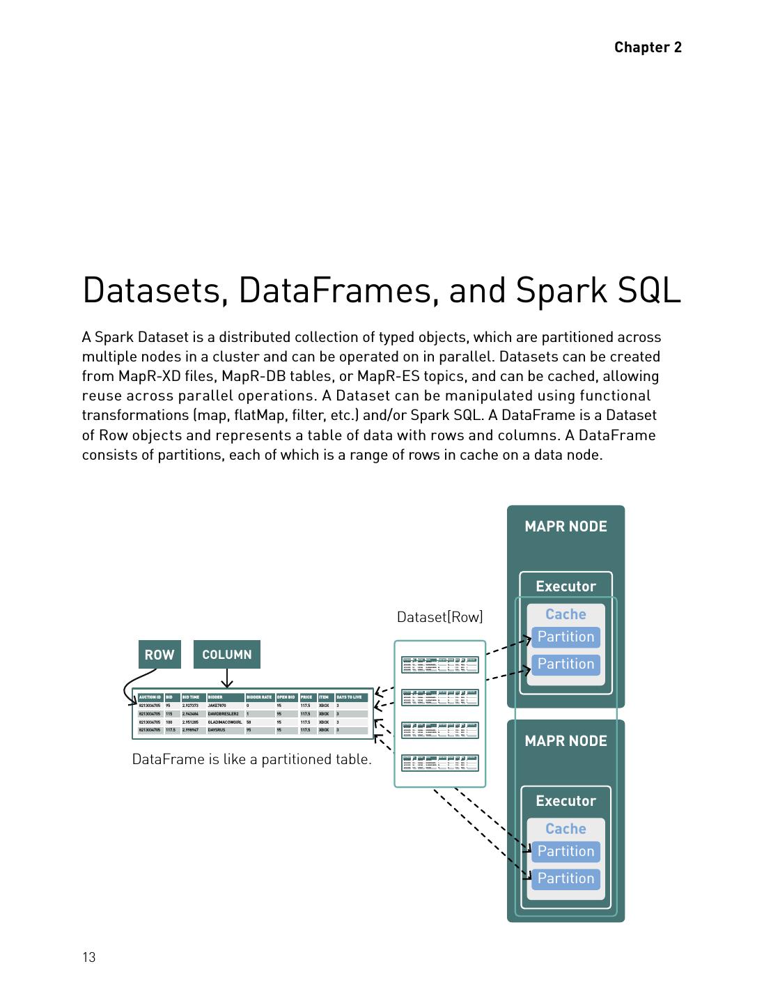
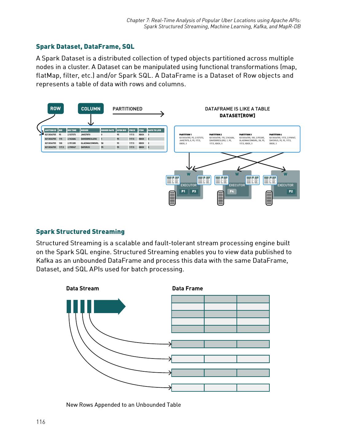
13 . Chapter 2 Datasets, DataFrames, and Spark SQL A Spark Dataset is a distributed collection of typed objects, which are partitioned across multiple nodes in a cluster and can be operated on in parallel. Datasets can be created from MapR-XD files, MapR-DB tables, or MapR-ES topics, and can be cached, allowing reuse across parallel operations. A Dataset can be manipulated using functional transformations (map, flatMap, filter, etc.) and/or Spark SQL. A DataFrame is a Dataset of Row objects and represents a table of data with rows and columns. A DataFrame consists of partitions, each of which is a range of rows in cache on a data node. MAPR NODE Executor Dataset[Row] Cache Partition ROW COLUMN Partition AUCTION ID BID BID TIME BIDDER BIDDER RATE OPEN BID PRICE ITEM DAYS TO LIVE 8213034705 95 2.927373 JAKE7870 0 95 117.5 XBOX 3 8213034705 115 2.943484 DAVIDBRESLER2 1 95 117.5 XBOX 3 8213034705 100 2.951285 GLADIMACOWGIRL 58 95 117.5 XBOX 3 8213034705 117.5 2.998947 DAYSRUS 95 95 117.5 XBOX 3 AUCTION ID BID BID TIME BIDDER BIDDER RATE OPEN BID PRICE ITEM DAYS TO LIVE 8213034705 95 2.927373 JAKE7870 0 95 117.5 XBOX 3 AUCTION ID BID BID TIME BIDDER BIDDER RATE OPEN BID PRICE ITEM DAYS TO LIVE 8213034705 8213034705 115 100 2.943484 2.951285 DAVIDBRESLER2 GLADIMACOWGIRL 1 58 95 95 117.5 117.5 XBOX XBOX 3 3 8213034705 117.5 2.998947 DAYSRUS 95 95 117.5 XBOX 3 8213034705 95 2.927373 JAKE7870 0 95 117.5 XBOX 3 8213034705 115 2.943484 DAVIDBRESLER2 1 95 117.5 XBOX 3 8213034705 100 2.951285 GLADIMACOWGIRL 58 95 117.5 XBOX 3 AUCTION ID BID BID TIME BIDDER BIDDER RATE OPEN BID PRICE ITEM DAYS TO LIVE 8213034705 95 2.927373 JAKE7870 0 95 117.5 XBOX 3 8213034705 117.5 2.998947 DAYSRUS 95 95 117.5 XBOX 3 MAPR NODE 8213034705 115 2.943484 DAVIDBRESLER2 1 95 117.5 XBOX 3 8213034705 100 2.951285 GLADIMACOWGIRL 58 95 117.5 XBOX 3 8213034705 117.5 2.998947 DAYSRUS 95 95 117.5 XBOX 3 DataFrame is like a partitioned table. AUCTION ID 8213034705 8213034705 8213034705 8213034705 BID 95 115 100 117.5 BID TIME 2.927373 2.943484 2.951285 2.998947 BIDDER JAKE7870 DAVIDBRESLER2 GLADIMACOWGIRL DAYSRUS BIDDER RATE 0 1 58 95 OPEN BID 95 95 95 95 PRICE 117.5 117.5 117.5 117.5 ITEM XBOX XBOX XBOX XBOX DAYS TO LIVE 3 3 3 3 Executor Cache Partition Partition 13
14 . Chapter 2: Datasets, DataFrames, and Spark SQL The SparkSession Object As discussed before, a Spark application runs as independent processes, coordinated by the SparkSession object in the driver program. The entry point to programming in Spark is the org.apache.spark.sql.SparkSession class, which you use to create a SparkSession object as shown below: val spark = SparkSession.builder().appName(“example”).master (“local[*]”).getOrCreate() If you are using the spark-shell or a notebook, the SparkSession object is already created and available as the variable Spark. Interactive Analysis with the Spark Shell The Spark shell provides an easy way to learn Spark interactively. You can start the shell with the following command: $ /[installation path]/bin/spark-shell --master local[2] You can enter the code from the rest of this chapter into the Spark shell; outputs from the shell are prefaced with result. Exploring U.S. Flight Data with Spark Datasets and DataFrames To go over some core concepts of Spark Datasets, we will be using some flight information from the United States Department of Transportation. Later, we will use this same data to predict flight delays, so we want to explore the flight attributes that most contribute to flight delays. Using Spark Datasets, we will explore the data to answer questions, like: which airline carriers, days of the week, originating airport, and hours of the day have the highest number of flight delays, when a delay is greater than 40 minutes. The flight data is in JSON files, with each flight having the following information: • id: ID composed of carrier, date, origin, destination, flight number • dofW: day of week (1=Monday, 7=Sunday) • carrier: carrier code • origin: origin airport code • dest: destination airport code • crsdephour: scheduled departure hour 14
15 . Chapter 2: Datasets, DataFrames, and Spark SQL • crsdeptime: scheduled departure time • depdelay: departure delay in minutes • crsarrtime: scheduled arrival time • arrdelay: arrival delay minutes • crselapsedtime: elapsed time • dist: distance It appears in the following format: { “_id”: “AA_2017-01-01_ATL_LGA_1678”, “dofW”: 7, “carrier”: “AA”, “origin”: “ATL”, “dest”: “LGA”, “crsdephour”: 17, “crsdeptime”: 1700, “depdelay”: 0.0, “crsarrtime”: 1912, “arrdelay”: 0.0, “crselapsedtime”: 132.0, “dist”: 762.0 } (The complete data and code for all examples are available in the GitHub link in the appendix.) 15
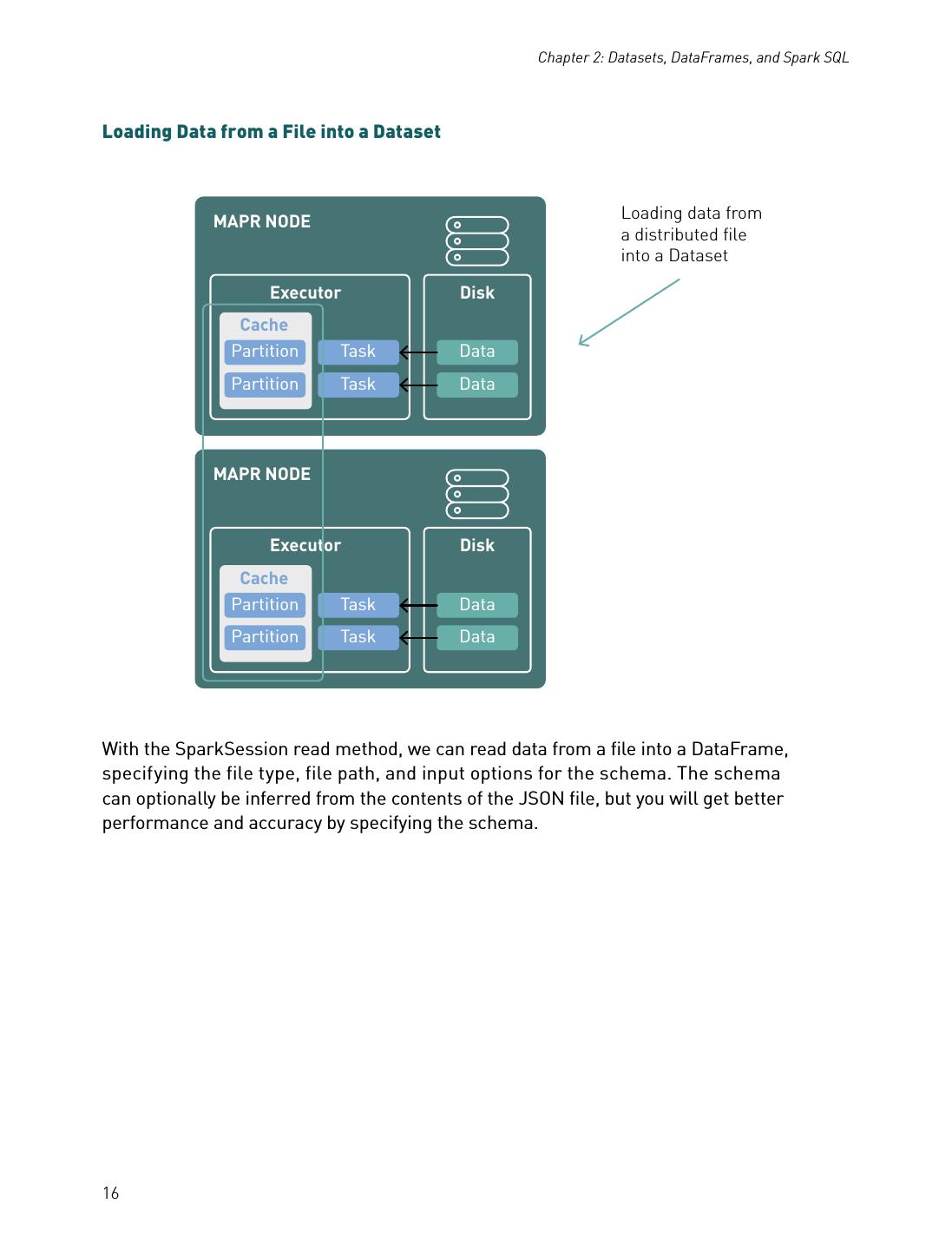
16 . Chapter 2: Datasets, DataFrames, and Spark SQL Loading Data from a File into a Dataset MAPR NODE Loading data from a distributed file into a Dataset Executor Disk Cache Partition Task Data Partition Task Data MAPR NODE Executor Disk Cache Partition Task Data Partition Task Data With the SparkSession read method, we can read data from a file into a DataFrame, specifying the file type, file path, and input options for the schema. The schema can optionally be inferred from the contents of the JSON file, but you will get better performance and accuracy by specifying the schema. 16
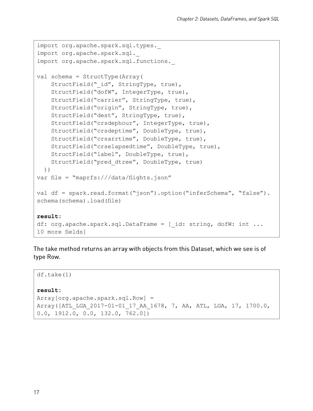
17 . Chapter 2: Datasets, DataFrames, and Spark SQL import org.apache.spark.sql.types._ import org.apache.spark.sql._ import org.apache.spark.sql.functions._ val schema = StructType(Array( StructField(“_id”, StringType, true), StructField(“dofW”, IntegerType, true), StructField(“carrier”, StringType, true), StructField(“origin”, StringType, true), StructField(“dest”, StringType, true), StructField(“crsdephour”, IntegerType, true), StructField(“crsdeptime”, DoubleType, true), StructField(“crsarrtime”, DoubleType, true), StructField(“crselapsedtime”, DoubleType, true), StructField(“label”, DoubleType, true), StructField(“pred_dtree”, DoubleType, true) )) var file = “maprfs:///data/flights.json” val df = spark.read.format(“json”).option(“inferSchema”, “false”). schema(schema).load(file) result: df: org.apache.spark.sql.DataFrame = [_id: string, dofW: int ... 10 more fields] The take method returns an array with objects from this Dataset, which we see is of type Row. df.take(1) result: Array[org.apache.spark.sql.Row] = Array([ATL_LGA_2017-01-01_17_AA_1678, 7, AA, ATL, LGA, 17, 1700.0, 0.0, 1912.0, 0.0, 132.0, 762.0]) 17
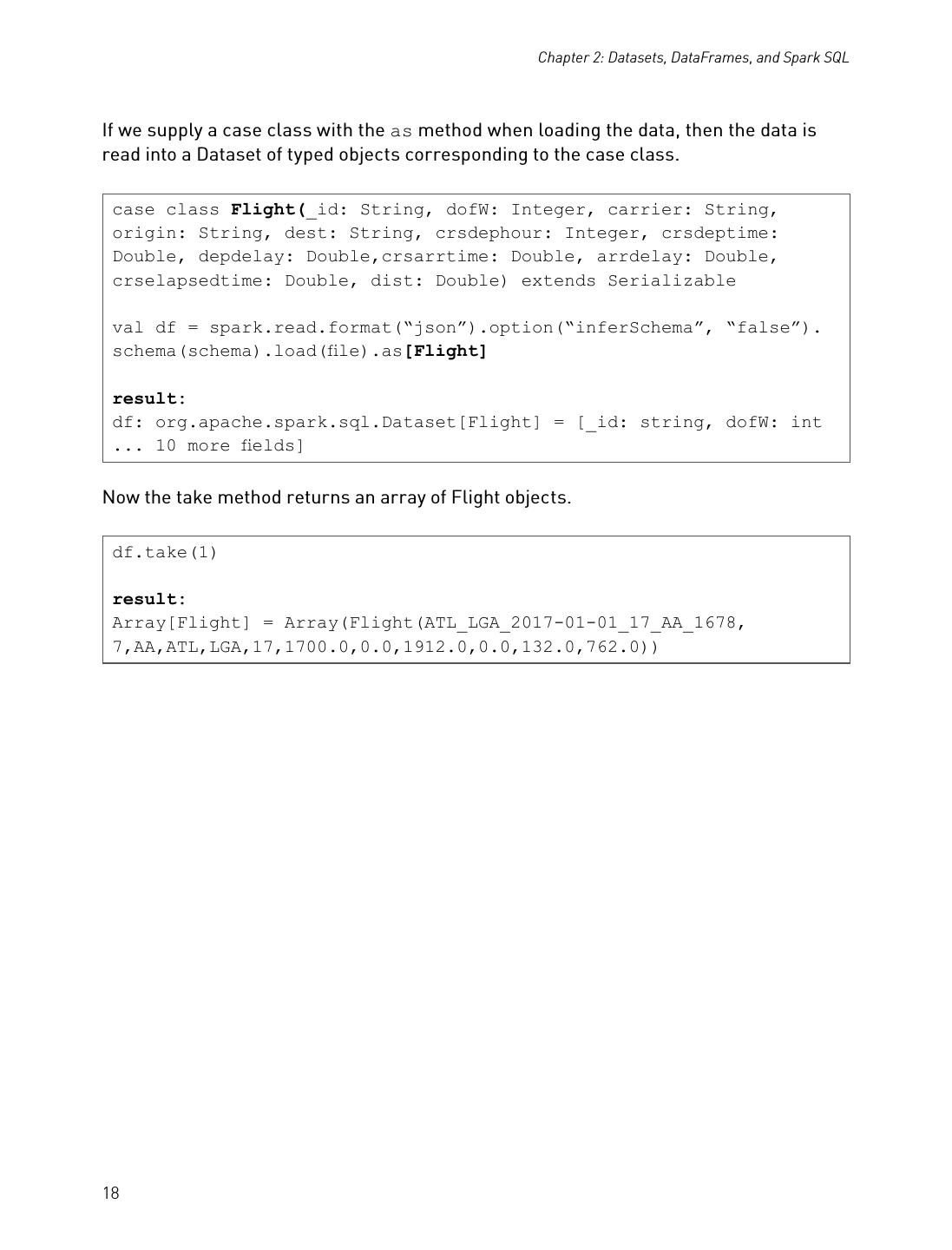
18 . Chapter 2: Datasets, DataFrames, and Spark SQL If we supply a case class with the as method when loading the data, then the data is read into a Dataset of typed objects corresponding to the case class. case class Flight(_id: String, dofW: Integer, carrier: String, origin: String, dest: String, crsdephour: Integer, crsdeptime: Double, depdelay: Double,crsarrtime: Double, arrdelay: Double, crselapsedtime: Double, dist: Double) extends Serializable val df = spark.read.format(“json”).option(“inferSchema”, “false”). schema(schema).load(file).as[Flight] result: df: org.apache.spark.sql.Dataset[Flight] = [_id: string, dofW: int ... 10 more fields] Now the take method returns an array of Flight objects. df.take(1) result: Array[Flight] = Array(Flight(ATL_LGA_2017-01-01_17_AA_1678, 7,AA,ATL,LGA,17,1700.0,0.0,1912.0,0.0,132.0,762.0)) 18
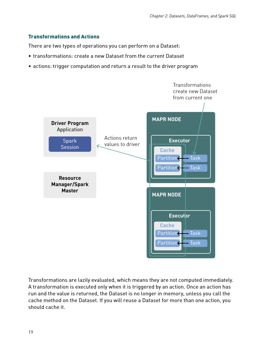
19 . Chapter 2: Datasets, DataFrames, and Spark SQL Transformations and Actions There are two types of operations you can perform on a Dataset: • transformations: create a new Dataset from the current Dataset • actions: trigger computation and return a result to the driver program Transformations create new Dataset from current one MAPR NODE Driver Program Application Actions return Executor Spark values to driver Session Cache Partition Task Partition Task Resource Manager/Spark Master MAPR NODE Executor Cache Partition Task Partition Task Transformations are lazily evaluated, which means they are not computed immediately. A transformation is executed only when it is triggered by an action. Once an action has run and the value is returned, the Dataset is no longer in memory, unless you call the cache method on the Dataset. If you will reuse a Dataset for more than one action, you should cache it. 19
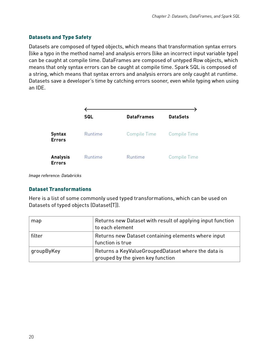
20 . Chapter 2: Datasets, DataFrames, and Spark SQL Datasets and Type Safety Datasets are composed of typed objects, which means that transformation syntax errors (like a typo in the method name) and analysis errors (like an incorrect input variable type) can be caught at compile time. DataFrames are composed of untyped Row objects, which means that only syntax errors can be caught at compile time. Spark SQL is composed of a string, which means that syntax errors and analysis errors are only caught at runtime. Datasets save a developer’s time by catching errors sooner, even while typing when using an IDE. SQL DataFrames DataSets Syntax Runtime Compile Time Compile Time Errors Analysis Runtime Runtime Compile Time Errors Image reference: (ImageDatabricks reference: Databricks) Dataset Transformations Here is a list of some commonly used typed transformations, which can be used on Datasets of typed objects (Dataset[T]). map Returns new Dataset with result of applying input function to each element filter Returns new Dataset containing elements where input function is true groupByKey Returns a KeyValueGroupedDataset where the data is grouped by the given key function 20
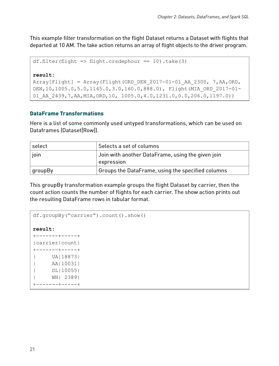
21 . Chapter 2: Datasets, DataFrames, and Spark SQL This example filter transformation on the flight Dataset returns a Dataset with flights that departed at 10 AM. The take action returns an array of flight objects to the driver program. df.filter(flight => flight.crsdephour == 10).take(3) result: Array[Flight] = Array(Flight(ORD_DEN_2017-01-01_AA_2300, 7,AA,ORD, DEN,10,1005.0,5.0,1145.0,3.0,160.0,888.0), Flight(MIA_ORD_2017-01- 01_AA_2439,7,AA,MIA,ORD,10, 1005.0,4.0,1231.0,0.0,206.0,1197.0)) DataFrame Transformations Here is a list of some commonly used untyped transformations, which can be used on Dataframes (Dataset[Row]). select Selects a set of columns join Join with another DataFrame, using the given join expression groupBy Groups the DataFrame, using the specified columns This groupBy transformation example groups the flight Dataset by carrier, then the count action counts the number of flights for each carrier. The show action prints out the resulting DataFrame rows in tabular format. df.groupBy(“carrier”).count().show() result: +-------+-----+ |carrier|count| +-------+-----+ | UA|18873| | AA|10031| | DL|10055| | WN| 2389| +-------+-----+ 21
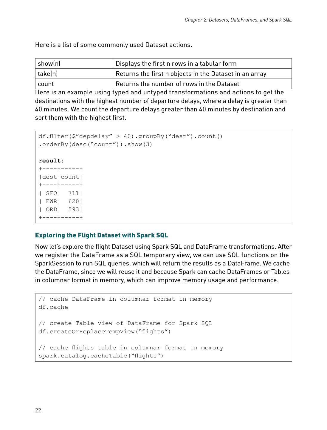
22 . Chapter 2: Datasets, DataFrames, and Spark SQL Here is a list of some commonly used Dataset actions. show(n) Displays the first n rows in a tabular form take(n) Returns the first n objects in the Dataset in an array count Returns the number of rows in the Dataset Here is an example using typed and untyped transformations and actions to get the destinations with the highest number of departure delays, where a delay is greater than 40 minutes. We count the departure delays greater than 40 minutes by destination and sort them with the highest first. df.filter($”depdelay” > 40).groupBy(“dest”).count() .orderBy(desc(“count”)).show(3) result: +----+-----+ |dest|count| +----+-----+ | SFO| 711| | EWR| 620| | ORD| 593| +----+-----+ Exploring the Flight Dataset with Spark SQL Now let’s explore the flight Dataset using Spark SQL and DataFrame transformations. After we register the DataFrame as a SQL temporary view, we can use SQL functions on the SparkSession to run SQL queries, which will return the results as a DataFrame. We cache the DataFrame, since we will reuse it and because Spark can cache DataFrames or Tables in columnar format in memory, which can improve memory usage and performance. // cache DataFrame in columnar format in memory df.cache // create Table view of DataFrame for Spark SQL df.createOrReplaceTempView(“flights”) // cache flights table in columnar format in memory spark.catalog.cacheTable(“flights”) 22
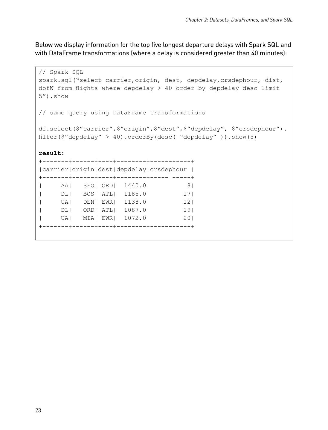
23 . Chapter 2: Datasets, DataFrames, and Spark SQL Below we display information for the top five longest departure delays with Spark SQL and with DataFrame transformations (where a delay is considered greater than 40 minutes): // Spark SQL spark.sql(“select carrier,origin, dest, depdelay,crsdephour, dist, dofW from flights where depdelay > 40 order by depdelay desc limit 5”).show // same query using DataFrame transformations df.select($”carrier”,$”origin”,$”dest”,$”depdelay”, $”crsdephour”). filter($”depdelay” > 40).orderBy(desc( “depdelay” )).show(5) result: +-------+------+----+--------+-----------+ |carrier|origin|dest|depdelay|crsdephour | +-------+------+----+--------+----- -----+ | AA| SFO| ORD| 1440.0| 8| | DL| BOS| ATL| 1185.0| 17| | UA| DEN| EWR| 1138.0| 12| | DL| ORD| ATL| 1087.0| 19| | UA| MIA| EWR| 1072.0| 20| +-------+------+----+--------+-----------+ 23
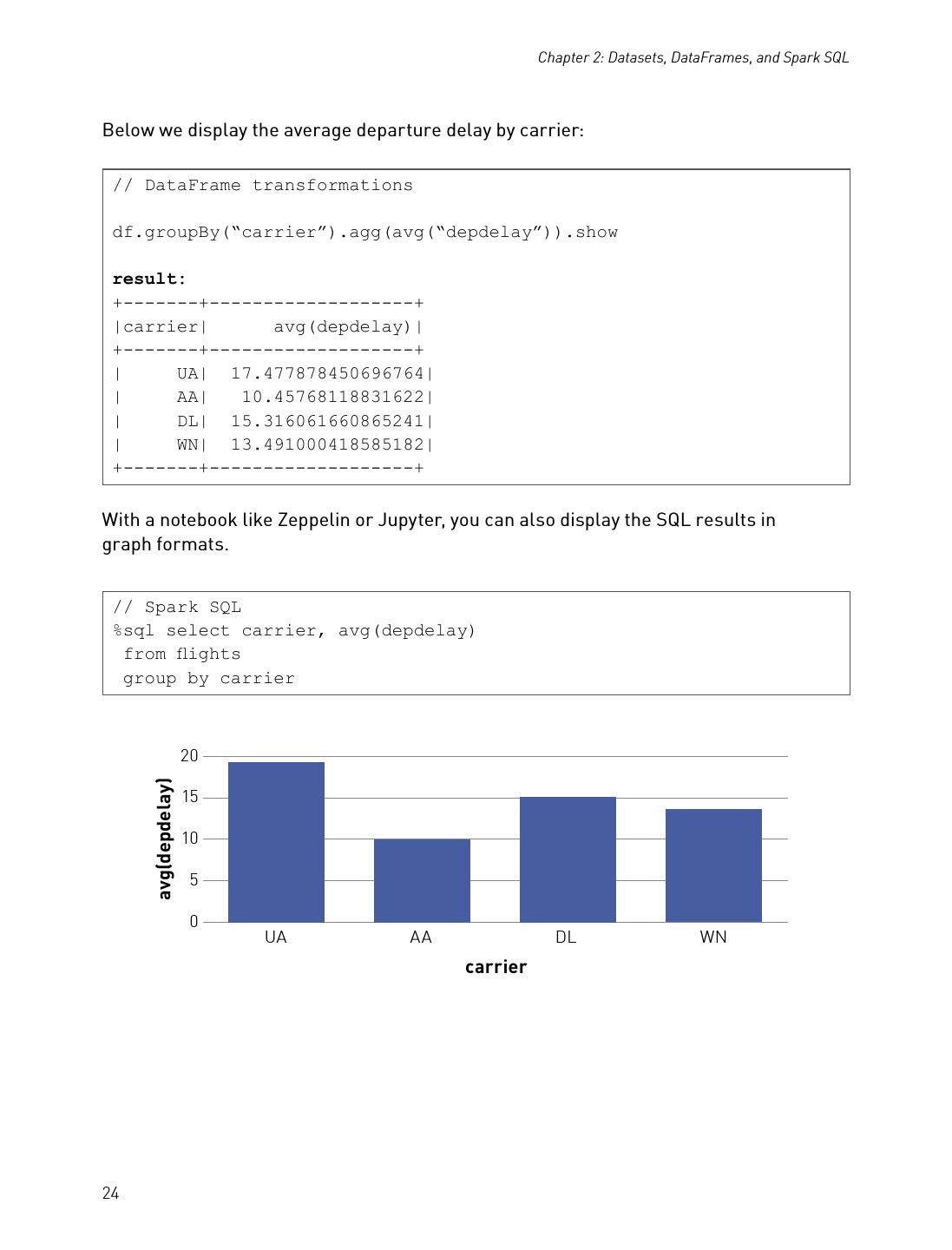
24 . Chapter 2: Datasets, DataFrames, and Spark SQL Below we display the average departure delay by carrier: // DataFrame transformations df.groupBy(“carrier”).agg(avg(“depdelay”)).show result: +-------+-------------------+ |carrier| avg(depdelay)| +-------+-------------------+ | UA| 17.477878450696764| | AA| 10.45768118831622| | DL| 15.316061660865241| | WN| 13.491000418585182| +-------+-------------------+ With a notebook like Zeppelin or Jupyter, you can also display the SQL results in graph formats. // Spark SQL %sql select carrier, avg(depdelay) from flights group by carrier 20 avg(depdelay) 15 10 5 0 UA AA DL WN carrier 24
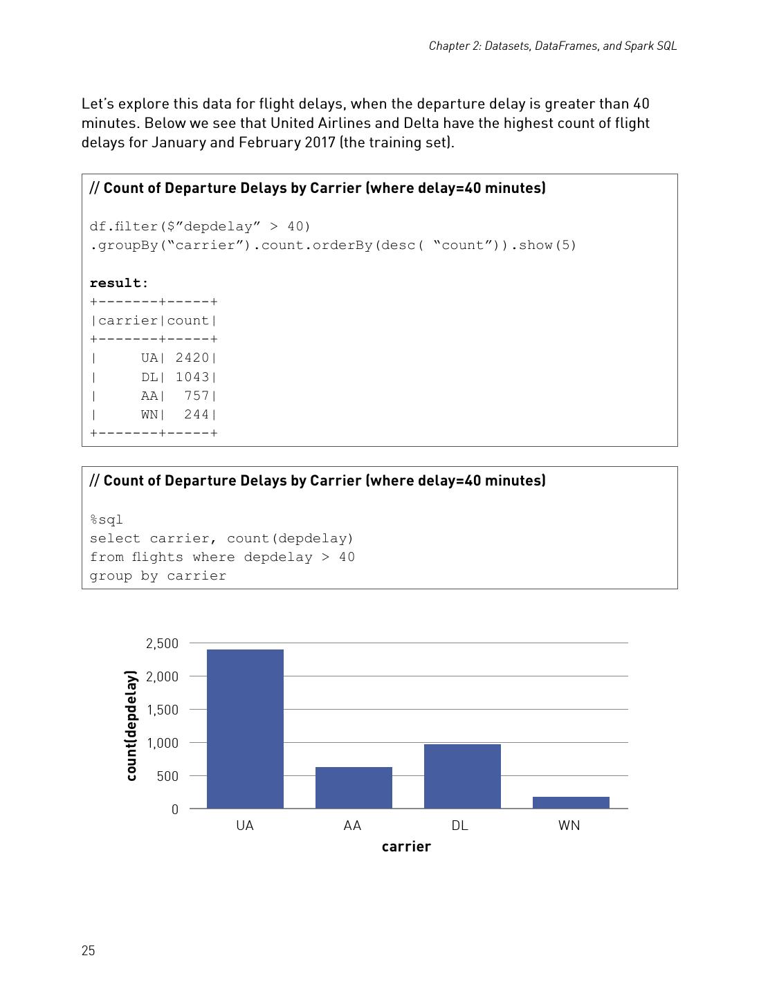
25 . Chapter 2: Datasets, DataFrames, and Spark SQL Let’s explore this data for flight delays, when the departure delay is greater than 40 minutes. Below we see that United Airlines and Delta have the highest count of flight delays for January and February 2017 (the training set). // Count of Departure Delays by Carrier (where delay=40 minutes) df.filter($”depdelay” > 40) .groupBy(“carrier”).count.orderBy(desc( “count”)).show(5) result: +-------+-----+ |carrier|count| +-------+-----+ | UA| 2420| | DL| 1043| | AA| 757| | WN| 244| +-------+-----+ // Count of Departure Delays by Carrier (where delay=40 minutes) %sql select carrier, count(depdelay) from flights where depdelay > 40 group by carrier 2,500 2,000 count(depdelay) 1,500 1,000 500 0 UA AA DL WN carrier 25
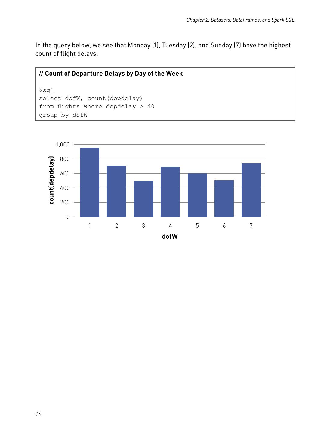
26 . Chapter 2: Datasets, DataFrames, and Spark SQL In the query below, we see that Monday (1), Tuesday (2), and Sunday (7) have the highest count of flight delays. // Count of Departure Delays by Day of the Week %sql select dofW, count(depdelay) from flights where depdelay > 40 group by dofW 1,000 800 count(depdelay) 600 400 200 0 1 2 3 4 5 6 7 dofW 26
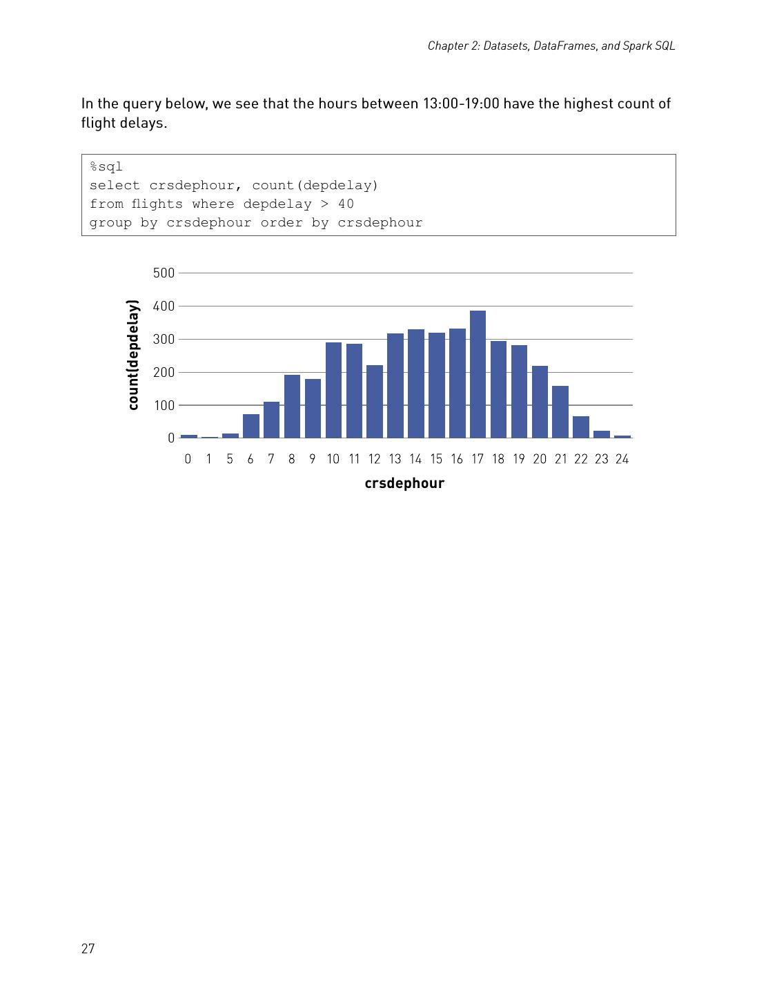
27 . Chapter 2: Datasets, DataFrames, and Spark SQL In the query below, we see that the hours between 13:00-19:00 have the highest count of flight delays. %sql select crsdephour, count(depdelay) from flights where depdelay > 40 group by crsdephour order by crsdephour 500 400 count(depdelay) 300 200 100 0 crsdephour 27
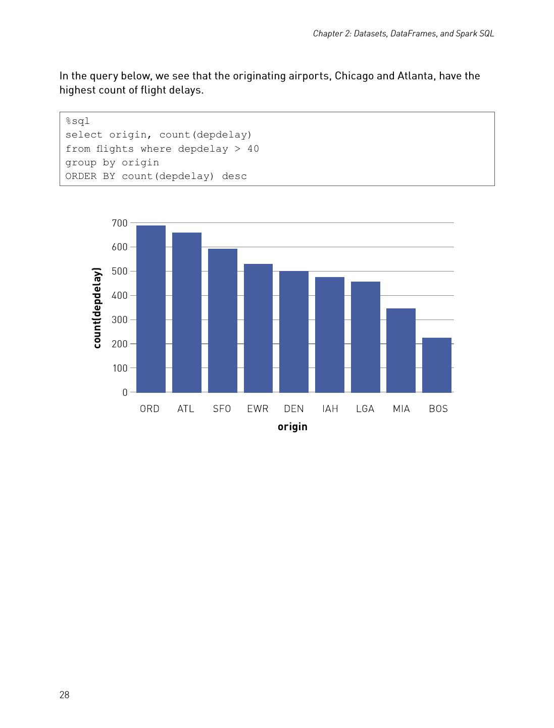
28 . Chapter 2: Datasets, DataFrames, and Spark SQL In the query below, we see that the originating airports, Chicago and Atlanta, have the highest count of flight delays. %sql select origin, count(depdelay) from flights where depdelay > 40 group by origin ORDER BY count(depdelay) desc 700 600 500 count(depdelay) 400 300 200 100 0 origin 28
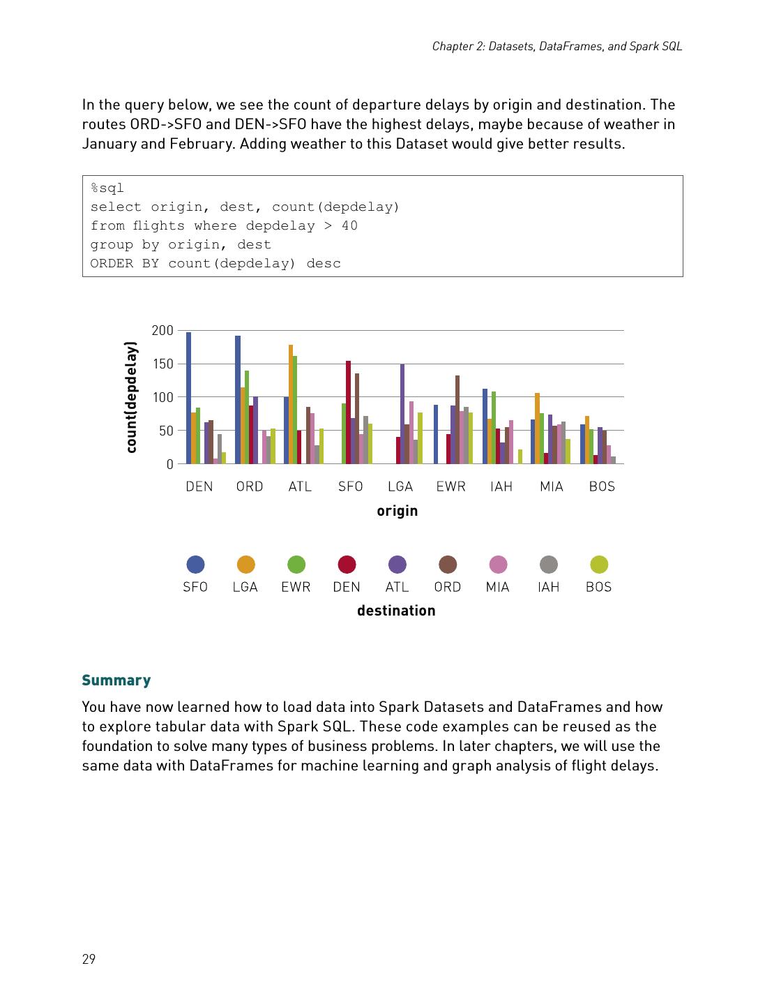
29 . Chapter 2: Datasets, DataFrames, and Spark SQL In the query below, we see the count of departure delays by origin and destination. The routes ORD->SFO and DEN->SFO have the highest delays, maybe because of weather in January and February. Adding weather to this Dataset would give better results. %sql select origin, dest, count(depdelay) from flights where depdelay > 40 group by origin, dest ORDER BY count(depdelay) desc 200 count(depdelay) 150 100 50 0 origin destination Summary You have now learned how to load data into Spark Datasets and DataFrames and how to explore tabular data with Spark SQL. These code examples can be reused as the foundation to solve many types of business problems. In later chapters, we will use the same data with DataFrames for machine learning and graph analysis of flight delays. 29


